---
title: "Analysis Notebook"
toc: true
toc-depth: 3
number-sections: true
fig-width: 6
fig-height: 6
execute:
freeze: false
cache: false
warning: false
message: false
---
This notebook contains all data processing, model fitting, and figure
generation code supporting the manuscript. All analyses can be reproduced
from the five CSV files in `data/derived/`. The rendered version of the
manuscript is available at the [project page](https://olivierraven.github.io/Koura_shoreline_habitats/).
# Setup
```{r}
#| label: setup
#| include: false
packages <- c(
  "DT","kableExtra","emmeans","patchwork","gratia","pROC","caret",
  "mgcv","glmmTMB","performance","tibble","tidyverse","readxl")

quiet_load <- function(pkg) {
  if (!requireNamespace(pkg, quietly = TRUE)) {
    suppressWarnings(suppressMessages(install.packages(pkg, dependencies = TRUE)))
  }
  suppressPackageStartupMessages(require(pkg, character.only = TRUE, quietly = TRUE))
  invisible(TRUE)
}

options(repos = c(CRAN = "https://cloud.r-project.org"))
invisible(lapply(packages, quiet_load))


exc_file_dir <- "data/raw/Natural_habitat.xlsx"
der_data_dir <- "data/derived"
out_dir      <- "outputs"

dir.create(exc_file_dir, showWarnings = FALSE, recursive = TRUE)
dir.create(der_data_dir, showWarnings = FALSE, recursive = TRUE)
dir.create(out_dir,      showWarnings = FALSE, recursive = TRUE)

Site_info          <- read_excel(exc_file_dir, sheet = "Site_info")
Monitoring_data    <- read_excel(exc_file_dir, sheet = "Monitoring_data")
Weed_data          <- read_excel(exc_file_dir, sheet = "Weed_data")  %>% dplyr::select(-starts_with("..."))
Fish_data <- read_excel(exc_file_dir, sheet = "Fish_data") %>% dplyr::select(-starts_with("..."))
Macroinvertebrates <- read_excel(exc_file_dir, sheet = "Macroinvertebrates")

Site_info          <- Site_info          |> dplyr::filter(!stringr::str_ends(monitoring_id, "_1"))
Monitoring_data    <- Monitoring_data    |> dplyr::filter(!stringr::str_ends(monitoring_id, "_1"))
Weed_data          <- Weed_data          |> dplyr::filter(!stringr::str_ends(monitoring_id, "_1"))
Fish_data          <- Fish_data          |> dplyr::filter(!stringr::str_ends(monitoring_id, "_1"))
Macroinvertebrates <- Macroinvertebrates |> dplyr::filter(!stringr::str_ends(monitoring_id, "_1"))

# Save as csv to derived
write.csv(Site_info,          file.path(der_data_dir, "Site_info.csv"),          row.names = FALSE)
write.csv(Monitoring_data,    file.path(der_data_dir, "Monitoring_data.csv"),    row.names = FALSE)
write.csv(Weed_data,          file.path(der_data_dir, "Weed_data.csv"),          row.names = FALSE)
write.csv(Fish_data,          file.path(der_data_dir, "Fish_data.csv"),          row.names = FALSE)
write.csv(Macroinvertebrates, file.path(der_data_dir, "Macroinvertebrates.csv"), row.names = FALSE)

# Reproducibility note ___________________________________________________
# The sections above require data/raw/Natural_habitat.xlsx (not tracked).
# To reproduce analyses and figures without the raw Excel file,
# run from here using the derived CSVs in data/derived/:

Site_info          <- read.csv(file.path(der_data_dir, "Site_info.csv"))
Monitoring_data    <- read.csv(file.path(der_data_dir, "Monitoring_data.csv"))
Weed_data          <- read.csv(file.path(der_data_dir, "Weed_data.csv"))
Fish_data          <- read.csv(file.path(der_data_dir, "Fish_data.csv"))
Macroinvertebrates <- read.csv(file.path(der_data_dir, "Macroinvertebrates.csv"))

# Set plot theme
base_theme_bw <- theme_classic() +
  theme(
    text = element_text(family = "Arial", size = 8),
    axis.title = element_text(face = "plain"),
    axis.text = element_text(face = "plain"),
    plot.title = element_text(face = "plain"),
    strip.text = element_text(face = "plain"),
    panel.border = element_rect(colour = "black", fill = NA, linewidth = 0.3)
  )

theme_set(base_theme_bw)

clean_smooth_title <- function(x) {
  x <- gsub("^s\\((.*)\\)$", "\\1", x)
  x <- gsub("_", " ", x)
  x
}

# Format of p values in text
format_pval <- function(p) {
  if (p < 0.001) {
    return("<0.001")
  } else {
    return(format(round(p, 3), nsmall = 3))
  }
}
```
# CPUE and BPUE derivation
## Length–weight model and predicted weights
```{r}
#| label: fig-length-weight
#| include: true
#| fig-width: 7
#| fig-height: 5
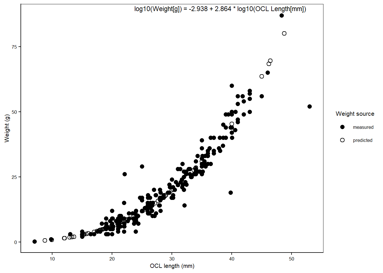
#| fig-cap: "Length–weight relationship used to estimate missing kōura weights. Observed (measured) and model-predicted body weights are shown in relation to orbital carapace length (OCL). The log₁₀–log₁₀ regression was fitted to individuals with both length and weight measurements (n = 240) and used to estimate missing weights (n = 81). Predicted values were back-transformed using a lognormal bias correction factor. The fitted regression equation is shown on the plot."
lw_model <- lm(
log10(weight_g) ~ log10(length_mm),
data = Fish_data,
subset = species_name == "Freshwater_crayfish" | maori_name == "Kōura",
na.action = na.exclude
)

sigma_log10 <- sigma(lw_model)
c <- 10^(0.5 * sigma_log10^2)

Fish_data <- Fish_data |>
mutate(
is_koura = species_name == "Freshwater_crayfish" | maori_name == "Kōura",
Predicted_weight = case_when(
!is.na(weight_g) ~ weight_g,
is_koura ~ {
pred_log <- predict(lw_model, newdata = pick(everything()))
10^(pred_log) * c
},
TRUE ~ NA_real_
),
Weight_source = case_when(
is_koura & !is.na(weight_g) ~ "measured",
is_koura & is.na(weight_g) ~ "predicted",
TRUE ~ NA_character_
)
)

a <- coef(lw_model)[1]
b <- coef(lw_model)[2]
formula_text <- paste0(
"log10(Weight[g]) = ", round(a, 3), " + ", round(b, 3),
" * log10(OCL Length[mm])"
)

length_weight_plot <- ggplot(
Fish_data |> dplyr::filter(is_koura),
aes(x = length_mm, y = Predicted_weight, shape = Weight_source)) +
geom_point(size = 2.2, colour = "black", stroke = 0.6) +
scale_shape_manual(values = c("measured" = 16, "predicted" = 1)) +
labs(x = "OCL length (mm)", y = "Weight (g)", shape = "Weight source") +
annotate("text", x = Inf, y = Inf, label = formula_text, hjust = 1.1, vjust = 1.3, size = 3)

ggsave(filename = file.path(out_dir, "fig-length-weight-ch3.png"), plot = length_weight_plot, width = 7, height = 5, dpi = 1200, create.dir = TRUE)

length_weight_plot
```
## CPUE and BPUE calculations
```{r}
#| label: cpue-bpue-calculations
#| include: false
CPUE_BPUE_legacy <- Fish_data %>%
filter(!is.na(species)) %>%
group_by(monitoring_id, species, net_type) %>%
dplyr::reframe(
Total_Individuals = sum(amount, na.rm = TRUE),
Total_Weight      = sum(Predicted_weight, na.rm = TRUE),
Total_Effort      = dplyr::first(amount_nets),
CPUE              = Total_Individuals / Total_Effort,
BPUE              = Total_Weight / Total_Effort,
Mean_Length       = mean(length_mm, na.rm = TRUE),
Min_Length        = ifelse(all(is.na(length_mm)), NA, min(length_mm, na.rm = TRUE)),
Max_Length        = ifelse(all(is.na(length_mm)), NA, max(length_mm, na.rm = TRUE)),
Mean_Weight       = mean(Predicted_weight, na.rm = TRUE),
Min_Weight        = ifelse(all(is.na(Predicted_weight)), NA, min(Predicted_weight, na.rm = TRUE)),
Max_Weight        = ifelse(all(is.na(Predicted_weight)), NA, max(Predicted_weight, na.rm = TRUE))
)

CPUE_BPUE_weighted <- CPUE_BPUE_legacy %>%
group_by(monitoring_id, species) %>%
summarise(
Total_Individuals       = sum(Total_Individuals, na.rm = TRUE),
Total_Weight            = sum(Total_Weight,      na.rm = TRUE),
Weighted_CPUE_numerator = sum(CPUE * Total_Effort,  na.rm = TRUE),
Weighted_BPUE_numerator = sum(BPUE * Total_Effort,  na.rm = TRUE),
Total_Effort_sum        = sum(Total_Effort,         na.rm = TRUE),
Mean_Length             = mean(Mean_Length, na.rm = TRUE),
Min_Length              = ifelse(all(is.na(Min_Length)), NA, min(Min_Length, na.rm = TRUE)),
Max_Length              = ifelse(all(is.na(Max_Length)), NA, max(Max_Length, na.rm = TRUE)),
Mean_Weight             = mean(Mean_Weight, na.rm = TRUE),
Min_Weight              = ifelse(all(is.na(Min_Weight)), NA, min(Min_Weight, na.rm = TRUE)),
Max_Weight              = ifelse(all(is.na(Max_Weight)), NA, max(Max_Weight, na.rm = TRUE)),
.groups = "drop"
) %>%
mutate(
Total_Effort_sum = ifelse(monitoring_id %in% c("96_0", "101_0", "117_1", "119_1"), 3, 4),
Weighted_CPUE    = Weighted_CPUE_numerator / Total_Effort_sum,
Weighted_BPUE    = Weighted_BPUE_numerator / Total_Effort_sum
)

species_presence_absence <- Fish_data %>%
filter(!is.na(species)) %>%
distinct(monitoring_id, species) %>%
mutate(Presence = 1) %>%
pivot_wider(
names_from  = species,
values_from = Presence,
values_fill = list(Presence = 0),
names_prefix = "Presence_"
) %>%
mutate(Predator_Fish_Presence = pmax(Presence_Trout, Presence_Eel, Presence_Catfish))

CPUE_BPUE_weighted_summary <- CPUE_BPUE_weighted %>%
pivot_wider(
names_from  = species,
values_from = c(
Total_Individuals, Weighted_CPUE, Weighted_BPUE, Total_Weight,
Mean_Length, Mean_Weight, Weighted_CPUE_numerator, Weighted_BPUE_numerator,
Total_Effort_sum, Min_Length, Max_Length, Min_Weight, Max_Weight
),
names_sep   = "_",
values_fill = list(Total_Individuals = 0, Weighted_CPUE = 0, Weighted_BPUE = 0)
) %>%
mutate(
Richness  = rowSums(dplyr::select(., starts_with("Total_Individuals_")) > 0),
Abundance = rowSums(dplyr::select(., starts_with("Total_Individuals_") & !ends_with(c("_Bullies", "_Common_smelt"))))
)
```
# Combined dataset and habitat classification
```{r}
#| label: combine-dataframes
#| include: false
unit_metadata <- Monitoring_data %>%
dplyr::select(parameter, unit) %>%
distinct()

Monitoring_summary <- Monitoring_data %>%
dplyr::select(-site_id, -group, -notes, -unit) %>%
pivot_wider(
names_from  = c(parameter),
values_from = value,
values_fill = list(value = NA)
) %>%
mutate(across(
c(
Bottom_visible, Water_clarity, Depth_10m, Slope, Riparian_vegetation, Vegetation_nearby,
Overhanging_trees, Erosion, Structure, Bedrock, Boulders, Cobble, Gravel,
Sand, Mud, Organic_matter, Rock_size, Temperature, DO_mgl, DO_percent,
Conductivity, Specific_conductivity, pH, Wood_cover
),
~ as.numeric(.)
))

Weed_summary <- Weed_data %>%
group_by(monitoring_id, weed_type, native_status) %>%
summarise(Total_Cover = sum(percentage_cover, na.rm = TRUE), .groups = "drop") %>%
pivot_wider(
names_from  = c(weed_type, native_status),
values_from = Total_Cover,
values_fill = 0
)

Macroinvertebrates_sum <- Macroinvertebrates %>%
group_by(monitoring_id, species) %>%
summarise(Total_amount = sum(amount, na.rm = TRUE), .groups = "drop") %>%
pivot_wider(names_from = c(species), values_from = Total_amount, values_fill = 0) %>%
mutate(
Invertebrates_Richness  = rowSums(dplyr::select(., -monitoring_id) > 0),
Invertebrates_Abundance = rowSums(dplyr::select(., -monitoring_id))
)

Monitoring_CPUE_data <- Site_info %>%
left_join(Monitoring_summary, by = "monitoring_id") %>%
left_join(
Weed_summary %>% dplyr::select(
monitoring_id,
Emergent_Native, Emergent_Non_Native,
Submerged_Native, Submerged_Non_Native, Turf_Native
),
by = "monitoring_id"
) %>%
left_join(CPUE_BPUE_weighted_summary, by = "monitoring_id") %>%
left_join(species_presence_absence, by = "monitoring_id") %>%
left_join(Macroinvertebrates_sum, by = "monitoring_id")

Monitoring_CPUE_data <- Monitoring_CPUE_data %>%
  mutate(
    Presence_rocks = if_else(Cobble > 1 | Boulders > 1, 1, 0),
    Slope_5m       = 5 / distance_5m,
    site_id_       = site_id - 60,
    monitoring_id_ = paste0(
      as.numeric(sub("_.*", "", monitoring_id)) - 60,
      sub("^[^_]*", "", monitoring_id)
    ),
    Monitoring     = sub(".*?_", "", monitoring_id),
    Date           = as.Date(date_time),
    Time           = format(as.POSIXct(date_time), "%H:%M:%S"),
    Year           = lubridate::year(date_time),
    Month          = lubridate::month(date_time, label = TRUE),
    Day            = lubridate::day(date_time),
    Season         = case_when(
      Month %in% c("Dec", "Jan", "Feb") ~ "Summer",
      Month %in% c("Mar", "Apr", "May") ~ "Autumn",
      Month %in% c("Jun", "Jul", "Aug") ~ "Winter",
      Month %in% c("Sep", "Oct", "Nov") ~ "Spring",
      TRUE ~ NA_character_
    ),
    Date_Time_Numeric = as.numeric(date_time)
  )
habitat_classification <- Monitoring_CPUE_data %>%
dplyr::select(
monitoring_id, DHT, lake,
Bedrock, Boulders, Cobble, Gravel, Sand, Mud, Organic_matter,
Emergent_Native, Emergent_Non_Native,
Submerged_Native, Submerged_Non_Native, Wood_cover
) %>%
pivot_longer(
cols = c(
Bedrock, Boulders, Cobble, Gravel, Sand, Mud, Organic_matter,
Emergent_Native, Emergent_Non_Native,
Submerged_Native, Submerged_Non_Native, Wood_cover
),
names_to = "Type",
values_to = "Percentage"
) %>%
group_by(monitoring_id) %>%
summarise(
Rocky_Percentage = sum(Percentage[Type %in% c("Bedrock", "Boulders", "Cobble")], na.rm = TRUE),
Sand_Percentage  = sum(Percentage[Type == "Sand"], na.rm = TRUE),
Mud_Percentage   = sum(Percentage[Type %in% c("Mud", "Organic_matter")], na.rm = TRUE),
Emergent_Percentage = sum(Percentage[Type == "Emergent_Native"], na.rm = TRUE),
Substrate_index = sum(
0.08 * Percentage[Type == "Bedrock"] +
0.07 * Percentage[Type == "Boulders"] +
0.06 * Percentage[Type == "Cobble"] +
0.04 * Percentage[Type == "Gravel"] +
0.03 * Percentage[Type == "Sand"] +
0.02 * Percentage[Type == "Organic_matter"] +
0.01 * Percentage[Type == "Mud"],
na.rm = TRUE
),
Substrate_CV = {
substrate_vals <- Percentage[Type %in% c("Bedrock", "Boulders", "Cobble", "Gravel", "Sand", "Mud", "Organic_matter")]
substrate_vals <- substrate_vals[!is.na(substrate_vals)]
if (length(substrate_vals) > 1 && mean(substrate_vals) > 0) {
sd(substrate_vals) / mean(substrate_vals)
} else {
NA_real_
}
},
.groups = "drop"
) %>%
mutate(
Habitat_Type = case_when(
Rocky_Percentage > 25 ~ "Rocky",
Emergent_Percentage > 25 ~ "Emergent Macrophyte",
Sand_Percentage >= Mud_Percentage ~ "Sandy",
TRUE ~ "Muddy"
)
) %>%
dplyr::select(monitoring_id, Habitat_Type, Substrate_index, Substrate_CV)

Monitoring_CPUE_data <- Monitoring_CPUE_data %>%
left_join(habitat_classification, by = "monitoring_id")

writexl::write_xlsx(Monitoring_CPUE_data, file.path(der_data_dir, "Monitoring_CPUE_data.xlsx"))
write.csv(Monitoring_CPUE_data, file.path(der_data_dir, "Monitoring_CPUE_data.csv"), row.names = FALSE)
write.csv(habitat_classification, file.path(der_data_dir, "habitat_classification.csv"), row.names = FALSE)

#head(Monitoring_CPUE_data)
```
## habitat-correlation
```{r}
#| label: habitat-correlation
#| include: false
cor(habitat_classification$Substrate_index,
habitat_classification$Substrate_CV,
use = "complete.obs")
```
# Lake overview table
```{r}
#| label: tbl-an-lake-overview
#| echo: false
#| tbl-cap: "Physical, morphometric, and trophic characteristics of the five Rotorua Te Arawa lakes surveyed, including sampling dates and number of littoral sites sampled per lake. Lake surface area, perimeter length, catchment area, depth, elevation, mixing regime, and trophic state for 2024 are derived from the @LAWA2025 database. Shoreline composition percentages are calculated from useable shoreline only, excluding geothermal and cliff sections."
shoreline_comp <- data.frame(
  `Lake name`                   = c("Rotorua", "Rotoiti", "Rotoehu", "Rotomā", "Ōkāreka"),
  `Muddy (%)`                   = c(0, 0, 3.3, 0, 8.9),
  `Sandy (%)`                   = c(82.8, 68.5, 91.2, 62.0, 45.1),
  `Rocky (%)`                   = c(17.2, 21.8, 1.7, 17.7, 20.2),
  `Emergent macrophytes (%)`    = c(0, 9.7, 3.8, 20.4, 25.8),
  check.names = FALSE
)

lake_data <- data.frame(
  `Lake name`                       = c("Rotorua", "Rotoiti", "Rotoehu", "Rotomā", "Ōkāreka"),
  `Sampling date (n sites)`         = c("20/02/2025 (12)", "15/01/2025 (12)", "10/12/2024 (12)", "6/11/2024 (12)", "31/10/2024 (10), 22/01/2025 (2)"),
  `Surface area (km²)`              = c(81, 34, 8, 11, 3),
  `Perimeter length (km)`           = c(45, 61, 40, 24, 11),
  `Catchment area (km²)`            = c(508, 123.7, 49.2, 27.8, 19.6),
  `Mean depth (m)`                  = c(11, 31.5, 8, 36.9, 20),
  `Maximum depth (m)`               = c(45, 124, 13.5, 83, 33.5),
  `Elevation (m)`                   = c(280, 279, 295, 316, 355),
  `Mixing regime`                   = c("Polymictic", "Monomictic", "Polymictic", "Monomictic", "Monomictic"),
  `Trophic state`                   = c("Eutrophic", "Mesotrophic", "Eutrophic", "Oligotrophic", "Mesotrophic"),
  check.names = FALSE
) %>%
  dplyr::left_join(shoreline_comp, by = "Lake name")

write.csv(lake_data, file = file.path(out_dir, "tbl-lake-overview.csv"), row.names = FALSE)

if (knitr::is_latex_output()) {
  col_nms <- colnames(lake_data)
  rotated_nms <- c(
    col_nms[1],
    sapply(col_nms[-1], function(x)
      paste0("\\rotatebox{90}{\\parbox{3.2cm}{\\raggedright ", x, "}}")
    )
  )
  knitr::kable(lake_data,
               booktabs = TRUE,
               col.names = rotated_nms,
               escape = FALSE,
               linesep = "") %>%
    kableExtra::kable_styling(
      latex_options = "hold_position",
      full_width = FALSE,
      font_size = 9
    ) %>%
    kableExtra::add_header_above(
      c(" " = 10, "Shoreline composition (%)" = 4),
      bold = TRUE
    ) %>%
    kableExtra::column_spec(1, width = "2.2cm") %>%
    kableExtra::column_spec(2, width = "1.8cm") %>%
    kableExtra::column_spec(3:14, width = "0.9cm")
} else {
  knitr::kable(lake_data)
}
```
# Overview of environmental and biotic variables
```{r}
#| label: tbl-an-environmental-biotic-overview
#| echo: false
#| tbl-cap: "Overview of environmental and biotic variables measured at littoral sampling sites, including variable descriptions, units, and hypothesised relevance for kōura (*Paranephrops planifrons*). Variables were selected a priori based on known habitat requirements, physiological constraints, and potential biotic interactions influencing kōura occurrence, abundance, and biomass in lake littoral zones."
biotic_vars <- data.frame(
  `Variable`= c("Lake identity", "Substrate index", "Slope", "Riparian vegetation", "Overhanging trees", "Wood cover", "Emergent and submerged macrophytes", "Temperature", "Dissolved oxygen", "Specific conductivity", "pH", "Fish presence"),
  `Description / Unit`= c("Categorical variable identifying lake", "Index based on % cover of bedrock, boulders, cobble, gravel, sand, mud, and organic matter", "Slope from shoreline to the 5 m depth contour", "Percentage cover of vegetation growing in the riparian zone", "Percentage cover of trees hanging over the shoreline", "Cover of wooden logs and tree branches in the sample site", "Percentage cover of macrophytes in the sample site divided over emergent and submerged and native and non-native species", "Temperature of surface water in °C", "Dissolved oxygen concentration in mg/L", "Electrical conductivity of the water in µS/cm", "Acidity or alkalinity of the water", "Presence/absence of selected native and non-native fish species"),
  `Hypothesised importance for kōura` = c("Captures unmeasured lake-specific differences in water chemistry, productivity, and catchment characteristics.", "Important for burrowing and shelter availability. Coarser substrates increase shelter availability through more crevices.", "Steeper slopes facilitate access to deeper water during daylight refuging and associate with coarser substrates.", "Contributes detrital inputs, bank stability, and shading at the water's edge.", "Provides direct shading and structural inputs into littoral habitats.", "Provides physical structure creating refuge spaces and supports macroinvertebrate prey availability.", "Native macrophytes can provide cover and serve as a food source. Non-native macrophytes may alter movement pathways and modify local habitat and water quality conditions.", "Influences metabolic rate, activity, physiological stress, and habitat suitability.", "Essential for respiration; reduced oxygen may constrain activity and habitat use.", "Reflects overall lake productivity, supporting food availability.", "Influences moulting success and exoskeleton strength, affected by acidity or calcium levels.", "Fish act as predators, competitors, or indirectly modify habitat structure."),
  `References` = c("Zuur et al., (2009)", "Usio & Townsend, (2000); Kusabs et al., (2015b)", "Devcich, (1979); Kusabs et al., (2015b)", "Parkyn et al., (2002)", "Smith et al., (1996); Vedia et al., (2017)", "Parkyn et al., (2009)", "Coffey & Clayton, (1988); Kusabs & Quinn, (2009)", "Devcich, (1979); Hammond et al., (2006); Parkyn & Collier, (2002); Angilletta et al., (2004)", "Hammond et al., (2006); Broughton et al., (2017)", "Devcich, (1979)", "Olsson et al., (2006)", "Shave et al., (1994); Barnes, (1996); Usio & Townsend, (2000); Barnes & Hicks, (2003)"),
  check.names = FALSE
)

write.csv(biotic_vars, file = file.path(out_dir, "tbl-environmental-biotic-overview.csv"), row.names = FALSE)

if (knitr::is_latex_output()) {
  knitr::kable(biotic_vars,
               booktabs = TRUE,
               longtable = TRUE,
               linesep = "") %>%
    kableExtra::kable_styling(
      latex_options = c("repeat_header"),
      font_size = 9,
      full_width = FALSE
    ) %>%
    kableExtra::column_spec(1, width = "2.5cm") %>%
    kableExtra::column_spec(2, width = "3.2cm") %>%
    kableExtra::column_spec(3, width = "5.8cm") %>%
    kableExtra::column_spec(4, width = "4.0cm")
} else {
  knitr::kable(biotic_vars)
}
```
# Environmental and fish summaries
```{r}
#| include: false
M_C_data <- Monitoring_CPUE_data
lake_order <- c("Rotorua", "Rotoiti", "Rotoehu", "Rotomā", "Ōkāreka")
M_C_data$lake <- factor(M_C_data$lake, levels = lake_order)

ci95 <- function(x) {
  x <- x[!is.na(x)]
  n <- length(x)
  if (n < 2) return(c(NA_real_, NA_real_))
  se <- sd(x) / sqrt(n)
  tcrit <- qt(0.975, df = n - 1)
  m <- mean(x)
  c(m - tcrit * se, m + tcrit * se)
}

unit_lookup <- Monitoring_data %>%
  dplyr::select(parameter, unit) %>%
  dplyr::distinct() %>%
  dplyr::mutate(
    Variable = dplyr::case_when(
      parameter == "Riparian_vegetation"       ~ "Riparian_vegetation",
      parameter == "Overhanging_trees"         ~ "Overhanging_trees",
      parameter == "Wood_cover"                ~ "Wood_cover",
      parameter == "Temperature"               ~ "Temperature",
      parameter == "DO_mgl"                    ~ "DO_mgl",
      parameter == "pH"                        ~ "pH",
      parameter == "Specific_conductivity"     ~ "Specific_conductivity",
      parameter == "Substrate_index"           ~ "Substrate_index",
      parameter == "Slope_5m"                  ~ "Slope_5m",
      TRUE ~ NA_character_
    )
  ) %>%
  dplyr::filter(!is.na(Variable)) %>%
  dplyr::select(Variable, unit) %>%
  dplyr::distinct()

# Add units for derived variables (not in Monitoring_data)
derived_units <- tibble::tibble(
  Variable = c("Emergent_vegetation", "Submerged_vegetation"),
  unit     = c("%", "%")
)

# Fish presence units (binary)
fish_units <- tibble::tibble(
  Variable = c(
    "Presence_Eel","Presence_Common_smelt","Presence_Catfish",
    "Presence_Goldfish","Presence_Kōaro","Presence_Trout"
  ),
  unit = ""
)

unit_lookup_all <- dplyr::bind_rows(unit_lookup, derived_units, fish_units) %>%
  dplyr::distinct(Variable, .keep_all = TRUE)

# ---- Environmental summary ----
Env_data <- M_C_data %>%
  dplyr::mutate(
    Emergent_vegetation  = Emergent_Native + Emergent_Non_Native,
    Submerged_vegetation = Submerged_Native + Submerged_Non_Native
  ) %>%
  dplyr::select(
    lake, Substrate_index, Slope_5m, Riparian_vegetation, Overhanging_trees, Wood_cover,
    Temperature, DO_mgl, pH, Specific_conductivity, Emergent_vegetation, Submerged_vegetation
  ) %>%
  tidyr::pivot_longer(-lake, names_to = "Variable", values_to = "Value")

Env_summary_table <- Env_data %>%
  dplyr::group_by(lake, Variable) %>%
  dplyr::summarise(
    n       = sum(!is.na(Value)),
    Mean    = mean(Value, na.rm = TRUE),
    Median  = median(Value, na.rm = TRUE),
    Min     = min(Value, na.rm = TRUE),
    Max     = max(Value, na.rm = TRUE),
    CI_low  = ci95(Value)[1],
    CI_high = ci95(Value)[2],
    .groups = "drop"
  )

Env_summary_all <- Env_data %>%
  dplyr::group_by(Variable) %>%
  dplyr::summarise(
    lake    = "All lakes",
    n       = sum(!is.na(Value)),
    Mean    = mean(Value, na.rm = TRUE),
    Median  = median(Value, na.rm = TRUE),
    Min     = min(Value, na.rm = TRUE),
    Max     = max(Value, na.rm = TRUE),
    CI_low  = ci95(Value)[1],
    CI_high = ci95(Value)[2],
    .groups = "drop"
  ) %>%
  dplyr::select(lake, dplyr::everything())

Env_summary_table <- dplyr::bind_rows(Env_summary_table, Env_summary_all)

# ---- Fish presence summary ----
Fish_data_long <- M_C_data %>%
  dplyr::select(
    lake, Presence_Eel, Presence_Common_smelt, Presence_Catfish,
    Presence_Goldfish, Presence_Kōaro, Presence_Trout
  ) %>%
  tidyr::pivot_longer(-lake, names_to = "Variable", values_to = "Presence")

Fish_summary_lake <- Fish_data_long %>%
  dplyr::group_by(lake, Variable) %>%
  dplyr::summarise(
    n       = sum(!is.na(Presence)),
    k       = sum(Presence, na.rm = TRUE),
    Mean    = mean(Presence, na.rm = TRUE),
    Median  = median(Presence, na.rm = TRUE),
    Min     = min(Presence, na.rm = TRUE),
    Max     = max(Presence, na.rm = TRUE),
    .groups = "drop"
  ) %>%
  dplyr::rowwise() %>%
  dplyr::mutate(
    CI_low  = ifelse(n > 0, binom.test(k, n)$conf.int[1], NA_real_),
    CI_high = ifelse(n > 0, binom.test(k, n)$conf.int[2], NA_real_)
  ) %>%
  dplyr::ungroup() %>%
  dplyr::select(-k)

Fish_summary_all <- Fish_data_long %>%
  dplyr::group_by(Variable) %>%
  dplyr::summarise(
    lake    = "All lakes",
    n       = sum(!is.na(Presence)),
    k       = sum(Presence, na.rm = TRUE),
    Mean    = mean(Presence, na.rm = TRUE),
    Median  = median(Presence, na.rm = TRUE),
    Min     = min(Presence, na.rm = TRUE),
    Max     = max(Presence, na.rm = TRUE),
    .groups = "drop"
  ) %>%
  dplyr::rowwise() %>%
  dplyr::mutate(
    CI_low  = ifelse(n > 0, binom.test(k, n)$conf.int[1], NA_real_),
    CI_high = ifelse(n > 0, binom.test(k, n)$conf.int[2], NA_real_)
  ) %>%
  dplyr::ungroup() %>%
  dplyr::select(lake, dplyr::everything(), -k)

Fish_summary_table <- dplyr::bind_rows(Fish_summary_lake, Fish_summary_all)

# ---- Combine + attach units + make Variable labels pretty ----
EnvBio_summary_table <- dplyr::bind_rows(Env_summary_table, Fish_summary_table) %>%
  dplyr::left_join(unit_lookup_all, by = "Variable") %>%
  dplyr::mutate(
    Variable = dplyr::recode(
      Variable,
      Substrate_index       = "Substrate index",
      Slope_5m              = "Slope 5m",
      Riparian_vegetation   = "Riparian vegetation",
      Overhanging_trees     = "Overhanging trees",
      Wood_cover            = "Wood cover",
      Emergent_vegetation   = "Emergent macrophytes",
      Submerged_vegetation  = "Submerged macrophytes",
      Temperature           = "Temperature",
      DO_mgl                = "Dissolved oxygen",
      Specific_conductivity = "Specific conductivity",
      pH                    = "pH",
      Presence_Catfish      = "Presence Catfish",
      Presence_Eel          = "Presence Eel",
      Presence_Goldfish     = "Presence Goldfish",
      Presence_Common_smelt = "Presence Common smelt",
      Presence_Kōaro        = "Presence Kōaro",
      Presence_Trout        = "Presence Trout"
    ),
    unit = dplyr::coalesce(unit, "")
  )

lake_order_exact <- c("Rotorua", "Rotoiti", "Rotoehu", "Rotomā", "Ōkāreka", "All lakes")

var_order_exact <- c("Substrate index","Slope 5m","Riparian vegetation","Overhanging trees","Wood cover","Emergent macrophytes", "Submerged macrophytes", "Temperature", "Dissolved oxygen", "Specific conductivity","pH", "Presence Catfish", "Presence Eel", "Presence Goldfish", "Presence Common smelt", "Presence Kōaro", "Presence Trout")

EnvBio_summary_table <- EnvBio_summary_table %>%
  dplyr::mutate(
    lake     = factor(as.character(lake), levels = lake_order_exact),
    Variable = factor(as.character(Variable), levels = var_order_exact)
  ) %>%
  dplyr::select(lake, Variable, unit, n, Mean, Median, Min, Max, CI_low, CI_high) %>%
  dplyr::arrange(Variable, lake) %>%
  dplyr::mutate(
    lake     = as.character(lake),
    Variable = as.character(Variable)
  )

# Save
write.csv(
  EnvBio_summary_table,
  file = file.path(out_dir, "tbl-env-fish-summary.csv"),
  row.names = FALSE
)
```
```{r}
#| label: tbl-an-env-fish-summary-widget
#| eval: !expr knitr::is_html_output()
#| include: !expr knitr::is_html_output()
#| tbl-cap: "Distribution of environmental and biotic variables measured at littoral sampling sites across five Te Arawa lakes in the Rotorua region of Aotearoa New Zealand."
DT::datatable(
  EnvBio_summary_table,
  filter = "top",
  options = list(
    pageLength = 20,
    dom = 'Bfrtip',
    buttons = c('csv', 'excel'),
    columnDefs = list(list(className = 'dt-center', targets = 3:9))
  ),
  extensions = 'Buttons',
  rownames = FALSE,
  colnames = c("Lake", "Variable", "Unit", "n", "Mean", "Median", "Min", "Max", "CI low", "CI high")
) |>
  DT::formatRound(columns = c("Mean","Median","Min","Max","CI_low","CI_high"), digits = 2)
```
```{r}
#| label: tbl-env-fish-summary-static
#| echo: false
#| eval: !expr "!knitr::is_html_output()"
#| tbl-cap: "Distribution of environmental and biotic variables measured at littoral sampling sites across five Te Arawa lakes in the Rotorua region of Aotearoa New Zealand."
knitr::kable(EnvBio_summary_table, digits = 2,
             align = c("l","l","l","r","r","r","r","r","r","r"),
             col.names = c("Lake","Variable","Unit","n","Mean","Median","Min","Max","CI low","CI high"))
```
# Kōura presence, CPUE, and BPUE across lakes
```{r}
#| label: fig-koura-by-lake
#| include: true
#| fig-width: 3
#| fig-height: 5
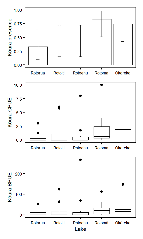
#| fig-cap: "Kōura presence, CPUE, and BPUE across lakes. The upper panel shows the proportion of sampled sites with kōura present in each lake, with error bars indicating 95% binomial confidence intervals. The middle and lower panels show the distribution of kōura CPUE and BPUE, respectively, across lakes using boxplots (median, interquartile range, and range)."
plot_koura_stats <- function(data, y_var, y_label,
type = c("continuous", "presence"),
show_x_title = FALSE) {

type <- match.arg(type)
lakes <- levels(data$lake)
xlab_text <- if (show_x_title) "Lake" else NULL

base_theme <- theme_classic() +
theme(
text = element_text(family = "Arial", size = 8),
axis.title = element_text(face = "plain"),
axis.text = element_text(face = "plain"),
panel.border = element_rect(colour = "black", fill = NA, linewidth = 0.3)
)

if (type == "continuous") {

ggplot(data, aes(lake, .data[[y_var]])) +
  geom_boxplot(fill = NA, colour = "black", linewidth = 0.3, outlier.size = 1.5) +
  scale_y_continuous(trans = "log1p",
    breaks = c(0, 1, 2, 5, 10, 25, 50, 100, 250),
    labels = scales::label_comma()) +
  labs(y = y_label, x = xlab_text) +
  base_theme
} else {
presence_summary <- data %>%
  group_by(lake) %>%
  summarise(
    n = sum(!is.na(.data[[y_var]])),
    k = sum(.data[[y_var]] == 1, na.rm = TRUE),
    Presence_Rate = ifelse(n > 0, k / n, NA_real_),
    .groups = "drop"
  ) %>%
  rowwise() %>%
  mutate(
    CI_low  = ifelse(n > 0, binom.test(k, n)$conf.int[1], NA_real_),
    CI_high = ifelse(n > 0, binom.test(k, n)$conf.int[2], NA_real_)
  ) %>%
  ungroup() %>%
  mutate(lake = factor(lake, levels = lakes))

ggplot(presence_summary, aes(x = lake, y = Presence_Rate)) +
  geom_col(fill = NA, colour = "black", linewidth = 0.3) +
  geom_errorbar(aes(ymin = CI_low, ymax = CI_high), width = 0.15, linewidth = 0.3) +
  scale_y_continuous(limits = c(0, 1)) +
  labs(x = xlab_text, y = y_label)
}
}

KPRES_plot <- plot_koura_stats(M_C_data, "Presence_Kōura", "Kōura presence", type = "presence", show_x_title = FALSE)
KCPUE_plot <- plot_koura_stats(M_C_data, "Weighted_CPUE_Kōura", "Kōura CPUE\n(log scale)", type = "continuous", show_x_title = FALSE)
KBPUE_plot <- plot_koura_stats(M_C_data, "Weighted_BPUE_Kōura", "Kōura BPUE\n(log scale)", type = "continuous", show_x_title = TRUE)

Koura_plots <- KPRES_plot / KCPUE_plot / KBPUE_plot

ggsave(file.path(out_dir, "fig-koura-by-lake.png"), Koura_plots,
       width = 3, height = 5, dpi = 1200)

Koura_plots
```
# Lake differences glmm
```{r}
#| label: lake-glmm
#| include: false
fit_presence_glmm <- function(data, response, lake_var = "lake", random_effect = "Habitat_Type") {
  form <- as.formula(paste0(response, " ~ ", lake_var, " + (1|", random_effect, ")"))
  glmmTMB::glmmTMB(form, data = data, family = binomial(link = "logit"))
}

fit_tweedie_glmm <- function(data, response, lake_var = "lake", random_effect = "Habitat_Type") {
  form <- as.formula(paste0(response, " ~ ", lake_var, " + (1|", random_effect, ")"))
  glmmTMB::glmmTMB(form, data = data, family = glmmTMB::tweedie(link = "log"))
}

m_koura_pres <- fit_presence_glmm(M_C_data, response = "Presence_Kōura",       lake_var = "lake", random_effect = "Habitat_Type")
m_koura_cpue <- fit_tweedie_glmm( M_C_data, response = "Weighted_CPUE_Kōura",  lake_var = "lake", random_effect = "Habitat_Type")
m_koura_bpue <- fit_tweedie_glmm( M_C_data, response = "Weighted_BPUE_Kōura",  lake_var = "lake", random_effect = "Habitat_Type")

# Overall lake effect (LRT via drop1)
pres_lrt <- drop1(m_koura_pres, test = "Chisq")
cpue_lrt <- drop1(m_koura_cpue, test = "Chisq")
bpue_lrt <- drop1(m_koura_bpue, test = "Chisq")

# Helper to report a drop1 LRT inline, e.g. "chi^2_4 = 13.76, p = 0.008"
report_lrt <- function(lrt_obj, term = "lake") {
  df    <- as.character(lrt_obj[term, "Df"])
  chisq <- formatC(lrt_obj[term, "LRT"], format = "f", digits = 2)
  p_val <- formatC(lrt_obj[term, "Pr(>Chi)"], format = "f", digits = 3)
  sprintf("$\\chi^2_{%s} = %s$, *p* = %s", df, chisq, p_val)
}

# Pairwise lake comparisons (BH-adjusted)
pres_pairs <- pairs(emmeans(m_koura_pres, ~ lake, type = "response"), adjust = "BH")
cpue_pairs <- pairs(emmeans(m_koura_cpue, ~ lake, type = "response"), adjust = "BH")
bpue_pairs <- pairs(emmeans(m_koura_bpue, ~ lake, type = "response"), adjust = "BH")

pres_lrt
cpue_lrt
bpue_lrt
```
# GAM modelling
### Helpers
```{r}
#| label: GAM-helpers
#| include: false
Modeling_data <- Monitoring_CPUE_data

alpha_sig    <- 0.1
p_cutoff_ml  <- 0.05
vif_thresh   <- 5
INCLUDE_RE   <- TRUE

custom_k <- list(
Slope_5m             = 10,
Riparian_vegetation  = 7,
Overhanging_trees    = 5,
Wood_cover           = 10,
Substrate_index      = 10,
Temperature          = 10,
pH                   = 10,
DO_mgl               = 10,
Emergent_Native      = 9,
Submerged_Non_Native = 9,
Turf_Native          = 6,
Submerged_Native     = 6
)

fish_vars <- c(
"Presence_Goldfish",
"Presence_Eel",
"Presence_Catfish",
"Presence_Common_smelt",
"Presence_Kōaro"
)

vars_common <- c(
"LID",
"Slope_5m","Riparian_vegetation","Overhanging_trees","Wood_cover","Substrate_index",
"Temperature","pH","DO_mgl","DO_percent","Specific_conductivity",
"Emergent_Native","Submerged_Non_Native","Turf_Native","Submerged_Native","Emergent_Non_Native",
fish_vars
)

is_cont <- function(x) is.numeric(x) && dplyr::n_distinct(x, na.rm = TRUE) >= 5

build_smooth_gam <- function(var, data, custom_k = list(), include_re_for_LID = FALSE) {
if (identical(var, "LID") && include_re_for_LID) return("s(LID, bs='re')")
x <- data[[var]]
if (is.numeric(x)) {
nuniq <- dplyr::n_distinct(x, na.rm = TRUE)
if (nuniq < 5) return(var)
k_req <- if (!is.null(custom_k[[var]])) custom_k[[var]] else 10
k_cap <- max(3, min(k_req, nuniq - 1))
return(paste0("s(", var, ", bs='ts', k=", k_cap, ")"))
}
var
}

exclude_if_RE <- function(mod){
if (!length(mod$smooth)) return(NULL)
has_re <- vapply(mod$smooth, function(s) "LID" %in% s$term, logical(1))
if (any(has_re)) "s(LID)" else NULL
}

remove_high_vif_glmBI <- function(
data,
response,
predictors,
threshold    = vif_thresh,
protect_vars = character(0),
verbose      = FALSE
) {
nzv <- caret::nearZeroVar(data[, predictors, drop = FALSE])
if (length(nzv)) predictors <- predictors[-nzv]

rpt <- list(removed = character(), start = predictors)
last_vif <- NULL

repeat {
if (!length(predictors)) stop("All predictors removed during VIF pruning.")


fml <- as.formula(paste(response, "~", paste(predictors, collapse = " + ")))
model <- try(lm(fml, data = data), silent = TRUE)
if (inherits(model, "try-error")) break

vif_data <- performance::check_collinearity(model)
vif_data <- vif_data[!grepl("\\|", vif_data$Term), , drop = FALSE]
last_vif <- vif_data

if (!nrow(vif_data) || all(vif_data$VIF < threshold)) break

ord <- order(vif_data$VIF, decreasing = TRUE)
to_remove <- NA_character_
for (i in ord) {
  cand <- vif_data$Term[i]
  if (!(cand %in% protect_vars)) { to_remove <- cand; break }
}
if (is.na(to_remove)) break

predictors  <- setdiff(predictors, to_remove)
rpt$removed <- c(rpt$removed, to_remove)
}

rpt$final_vif <- last_vif
list(predictors = predictors, report = rpt)
}

remove_high_vif_glmmTMB <- function(
data,
response,
predictors,
threshold    = vif_thresh,
protect_vars = character(0),
verbose      = FALSE
) {
nzv <- caret::nearZeroVar(data[, predictors, drop = FALSE])
if (length(nzv)) predictors <- predictors[-nzv]

rpt <- list(removed = character(), start = predictors)
last_vif <- NULL

repeat {
if (!length(predictors)) stop("All predictors removed during VIF pruning.")


fml <- as.formula(paste(response, "~", paste(predictors, collapse = " + ")))
model <- try(lm(fml, data = data), silent = TRUE)
if (inherits(model, "try-error")) break

vif_data <- performance::check_collinearity(model)
vif_data <- vif_data[!grepl("\\|", vif_data$Term), , drop = FALSE]
last_vif <- vif_data

if (!nrow(vif_data) || all(vif_data$VIF < threshold)) break

ord <- order(vif_data$VIF, decreasing = TRUE)
to_remove <- NA_character_
for (i in ord) {
  cand <- vif_data$Term[i]
  if (!(cand %in% protect_vars)) { to_remove <- cand; break }
}
if (is.na(to_remove)) break

predictors  <- setdiff(predictors, to_remove)
rpt$removed <- c(rpt$removed, to_remove)

}

rpt$final_vif <- last_vif
list(predictors = predictors, report = rpt)
}

as_plot <- function(p) if (inherits(p, c("gg","ggplot","patchwork"))) p else patchwork::plot_spacer()

prepare_block <- function(Modeling_data, response, vars_common, id = "LID"){
vars <- c(response, vars_common)
Modeling_data %>%
dplyr::select(dplyr::all_of(vars)) %>%
dplyr::mutate(
"{id}" := factor(.data[[id]]),
dplyr::across(dplyr::any_of(fish_vars), ~ as.numeric(.x))
)
}

ref_row <- function(data){
dplyr::summarise(
data,
dplyr::across(
dplyr::everything(),
\(x){
if (is.numeric(x)) stats::median(x, na.rm = TRUE)
else if (is.factor(x)) levels(x)[1L]
else if (is.logical(x)) FALSE
else if (is.character(x)) unique(stats::na.omit(x))[1L]
else x[1L]
}
)
)
}

is_binary_numeric <- function(x) is.numeric(x) && dplyr::n_distinct(x, na.rm = TRUE) == 2

get_term_p <- function(m, var, kind = c("any","param","smooth")){
kind <- match.arg(kind)
sm <- summary(m)

if (kind %in% c("any","param")) {
if (!is.null(sm$p.table) && nrow(sm$p.table) > 0) {
pcol <- intersect(colnames(sm$p.table), c("Pr(>|t|)","Pr(>|z|)"))[1]
if (!is.na(pcol) && var %in% rownames(sm$p.table)) {
return(as.numeric(sm$p.table[var, pcol]))
}
}
}

if (kind %in% c("any","smooth")) {
if (!is.null(sm$s.table) && nrow(sm$s.table) > 0) {
sname <- paste0("s(", var, ")")
if (sname %in% rownames(sm$s.table)) {
return(as.numeric(sm$s.table[sname, "p-value"]))
}
}
}

NA_real_
}

plot_binary_single_component <- function(model, var, data,
family = c("binomial","gamma"),
S = 2000, alpha = 0.05,
exclude_RE = TRUE,
hold_binaries = c("mean","zero","one"),
id = "LID",
fish_covars = c("Presence_Goldfish","Presence_Eel","Presence_Catfish","Presence_Common_smelt"),
seed = 1) {
family <- match.arg(family)
hold_binaries <- match.arg(hold_binaries)

tl <- attr(terms(model), "term.labels")
has_term <- any(tl == var) || any(grepl(paste0("^s\\(", var, "(,|\\))"), tl))
if (!has_term) return(ggplot() + theme_void())

num_means <- data %>%
dplyr::summarise(across(where(is.numeric), ~ mean(.x, na.rm = TRUE)))
base <- as.list(num_means)
if (id %in% names(data) && is.factor(data[[id]]))
base[[id]] <- factor(levels(data[[id]])[1], levels = levels(data[[id]]))

others <- setdiff(intersect(fish_covars, names(data)), var)
set_bin <- function(x){
if (hold_binaries == "mean") round(mean(data[[x]], na.rm = TRUE))
else if (hold_binaries == "zero") 0L else 1L
}
for (x in others) base[[x]] <- set_bin(x)

mk_nd <- function(level){
nd <- as.data.frame(base, stringsAsFactors = FALSE)
nd[[var]] <- as.integer(level)
if (id %in% names(data) && is.factor(data[[id]])) {
nd <- do.call(
rbind,
lapply(levels(data[[id]]), function(lv){
r <- nd
r[[id]] <- factor(lv, levels = levels(data[[id]]))
r
})
)
}
if (!is.null(model$model)) {
common <- intersect(names(nd), names(model$model))
for (nm in common) if (is.factor(model$model[[nm]]))
nd[[nm]] <- factor(nd[[nm]], levels = levels(model$model[[nm]]))
}
nd
}
nd0 <- mk_nd(0L)
nd1 <- mk_nd(1L)
nd  <- dplyr::bind_rows(
dplyr::mutate(nd0, .level = 0L),
dplyr::mutate(nd1, .level = 1L)
)

excl <- if (exclude_RE) exclude_if_RE(model) else NULL
lp <- predict(model, newdata = nd, type = "link", se.fit = TRUE, exclude = excl)

set.seed(seed)
n <- nrow(nd)
Z <- matrix(
rnorm(n * S, lp$fit, pmax(lp$se.fit, .Machine$double.eps)),
nrow = n, ncol = S
)

if (family == "binomial") {
Y <- plogis(Z); ylab <- "Presence probability"
} else {
Y <- exp(Z);    ylab <- "Mean given presence (μ)"
}

sim_by_level <- function(level_flag){
sims <- Y[nd$.level == level_flag, , drop = FALSE]
colMeans(sims)
}
sim0 <- sim_by_level(0L)
sim1 <- sim_by_level(1L)

qlo <- alpha/2
qhi <- 1 - alpha/2
df <- data.frame(
level = factor(c(0,1), levels = c(0,1), labels = c("Absent","Present")),
mean  = c(mean(sim0), mean(sim1)),
lwr   = c(quantile(sim0, qlo), quantile(sim1, qlo)),
upr   = c(quantile(sim0, qhi), quantile(sim1, qhi))
)

ggplot(df, aes(x = level, y = mean)) +
geom_col(width = 0.6) +
geom_errorbar(aes(ymin = lwr, ymax = upr), width = 0.2) +
labs(x = var, y = ylab)
}

plot_linear_single_component <- function(model, var, data,
family = c("binomial","gamma"),
n = 100, alpha = 0.05,
exclude_RE = TRUE) {
family <- match.arg(family)

num_means <- data %>%
dplyr::summarise(across(where(is.numeric), ~ mean(.x, na.rm = TRUE)))
base <- as.list(num_means)

if (!is.null(model$model)) {
for (nm in names(model$model)) {
if (is.factor(model$model[[nm]])) {
base[[nm]] <- factor(
levels(model$model[[nm]])[1],
levels = levels(model$model[[nm]])
)
}
}
}

x  <- data[[var]]
xr <- range(x, na.rm = TRUE)
grid <- seq(xr[1], xr[2], length.out = n)

nd <- as.data.frame(base)
nd <- nd[rep(1, n), , drop = FALSE]
nd[[var]] <- grid

excl <- if (exclude_RE) exclude_if_RE(model) else NULL
pr <- predict(model, newdata = nd, type = "link", se.fit = TRUE, exclude = excl)

if (family == "binomial") {
fit <- plogis(pr$fit)
lwr <- plogis(pr$fit - qnorm(1 - alpha/2) * pr$se.fit)
upr <- plogis(pr$fit + qnorm(1 - alpha/2) * pr$se.fit)
ylab <- "Response (probability)"
} else {
fit <- exp(pr$fit)
lwr <- exp(pr$fit - qnorm(1 - alpha/2) * pr$se.fit)
upr <- exp(pr$fit + qnorm(1 - alpha/2) * pr$se.fit)
ylab <- "Response (μ)"
}

df <- data.frame(x = grid, fit = fit, lwr = lwr, upr = upr)
ggplot(df, aes(x, fit)) +
geom_ribbon(aes(ymin = lwr, ymax = upr), alpha = 0.2) +
geom_line() +
labs(x = var, y = ylab)
}

parametric_panel <- function(model, data, alpha = 0.1, exclude = character(0),
family = c("binomial","gamma"),
fish_covars = c("Presence_Goldfish","Presence_Eel","Presence_Catfish","Presence_Common_smelt"),
hold_binaries = "mean") {
family <- match.arg(family)

sm <- summary(model)
if (is.null(sm$p.table) || nrow(sm$p.table) == 0) return(ggplot() + theme_void())

pcol <- intersect(colnames(sm$p.table), c("Pr(>|t|)","Pr(>|z|)"))[1]
if (is.na(pcol)) return(ggplot() + theme_void())

par_names <- setdiff(rownames(sm$p.table), "(Intercept)")

smooth_rows <- if (!is.null(sm$s.table)) rownames(sm$s.table) else character(0)
smooth_vars <- sub("^s\\(([^,\\)]+).*$", "\\1", smooth_rows)
par_names <- setdiff(par_names, union(exclude, smooth_vars))

par_sig <- par_names[sm$p.table[par_names, pcol, drop = TRUE] <= alpha]
if (!length(par_sig)) return(ggplot() + theme_void())

plots <- lapply(par_sig, function(v) {
x <- data[[v]]
if (is.null(x)) return(ggplot() + theme_void())

is_bin_num <- is.numeric(x) && dplyr::n_distinct(x, na.rm = TRUE) <= 2
is_bin_fac <- is.factor(x)  && nlevels(x) == 2

if (is_bin_num || is_bin_fac) {
plot_binary_single_component(
model, v, data,
family        = family,
hold_binaries = hold_binaries,
fish_covars   = fish_covars
)
} else {
plot_linear_single_component(model, v, data, family = family)
}
})

if (!length(plots)) return(ggplot() + theme_void())
patchwork::wrap_plots(plots, ncol = 1)
}
```
## Occupancy model (presence/absence)
Binomial GAMM with logit link. Stepwise backward elimination using ML
estimation (α = 0.05), refitted with REML. Lake identity (LID) included
as a random effect throughout and protected from removal.
### Model fitting
```{r}
#| label: occupancy-model
#| include: false
PData <- prepare_block(Modeling_data, "Presence_Kōura", vars_common)

id <- "LID"
pred_fixed_occ <- setdiff(names(PData), c("Presence_Kōura", id))

vif_occ <- remove_high_vif_glmBI(
PData,
"Presence_Kōura",
pred_fixed_occ,
threshold    = vif_thresh,
protect_vars = character(0)
)
kept_fixed_occ <- vif_occ$predictors

vars_step_occ <- c(kept_fixed_occ, if (INCLUDE_RE) id)
rhs_full_occ <- paste(
vapply(
vars_step_occ,
function(v) build_smooth_gam(v, PData, custom_k, include_re_for_LID = INCLUDE_RE),
character(1)
),
collapse = " + "
)
form_full_occ <- as.formula(paste("Presence_Kōura ~", rhs_full_occ))


full_ml_occ <- mgcv::gam(
  form_full_occ,
  data   = PData,
  family = binomial(link = "logit"),
  method = "ML",
  select = TRUE
)

remaining_occ <- vars_step_occ
protected_step_vars <- if (INCLUDE_RE) id else character(0)

repeat {
rhs_now <- paste(
vapply(
remaining_occ,
function(v) build_smooth_gam(v, PData, custom_k, include_re_for_LID = INCLUDE_RE),
character(1)
),
collapse = " + "
)
m_now <- mgcv::gam(
as.formula(paste("Presence_Kōura ~", rhs_now)),
data   = PData,
family = binomial(link = "logit"),
method = "ML",
select = TRUE
)
sm <- summary(m_now)

ps <- c()
if (!is.null(sm$p.table) && nrow(sm$p.table) > 0) {
pcol <- intersect(colnames(sm$p.table), c("Pr(>|t|)","Pr(>|z|)"))[1]
pvec <- sm$p.table[, pcol]
ps <- c(ps, pvec[names(pvec) != "(Intercept)"])
}
if (!is.null(sm$s.table) && nrow(sm$s.table) > 0) {
pvec <- sm$s.table[, "p-value"]
names(pvec) <- rownames(sm$s.table)
ps <- c(ps, pvec)
}
drop_candidates <- ps[ps > p_cutoff_ml]
if (!length(drop_candidates)) { red_ml_occ <- m_now; break }

ordered <- names(sort(drop_candidates, decreasing = TRUE))
ordered_vars <- vapply(
ordered,
function(x) if (grepl("^s\\(", x)) sub("^s\\(([^,]+).*\\)$", "\\1", x) else x,
character(1)
)

ordered_vars <- setdiff(ordered_vars, protected_step_vars)
if (!length(ordered_vars)) { red_ml_occ <- m_now; break }

remove_v <- ordered_vars[1]
remaining_occ <- setdiff(remaining_occ, remove_v)
if (!length(remaining_occ)) { red_ml_occ <- m_now; break }
}

final_occ <- mgcv::gam(
formula(red_ml_occ),
data   = PData,
family = binomial(link = "logit"),
method = "REML",
select = TRUE
)
```
### Model diagnostics
```{r}
#| label: occ-diagnostics
#| include: true
# Basis dimension check and residual diagnostics
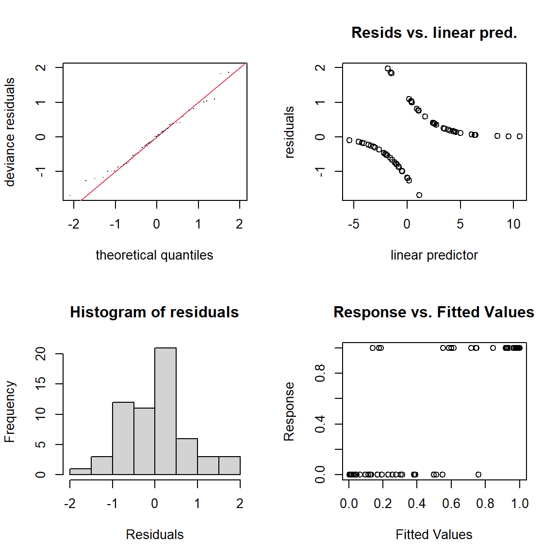
gam.check(final_occ)
```
```{r}
#| label: occ-concurvity
#| include: true
# Concurvity — values approaching 1 indicate potential instability
concurvity(final_occ, full = FALSE)
```
### Model figure
```{r}
#| label: fig-occupancy-model
#| include: true
#| fig-width: 7
#| fig-height: 5
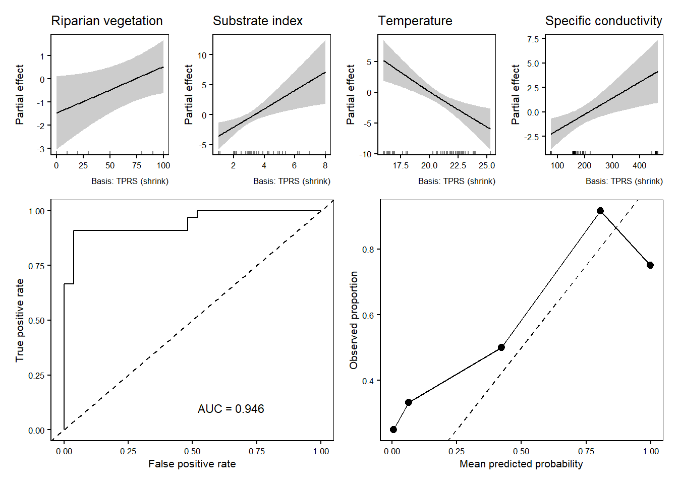
#| fig-cap: "Kōura occupancy GAMM results and model performance. (A) Estimated smooth terms for riparian vegetation, substrate index, surface water temperature, and specific conductivity, shown as partial effects with 95% confidence intervals. See Fig. S2 for raw data underlying modelled relationships. (B) Receiver operating characteristic (ROC) curve illustrating model discrimination, with the area under the curve (AUC) reported. (C) Calibration plot based on five equal-frequency bins, comparing mean predicted occupancy probabilities with observed proportions of occupied sites; the dashed 1:1 line indicates perfect calibration."
# Smooth plots: keep draw() outputs as-is (they may be ggplot OR patchwork)
sm <- gratia::smooth_estimates(final_occ)
smooth_names <- unique(sm$.smooth)
smooth_4_names <- smooth_names[1:min(4, length(smooth_names))]

plots_4 <- lapply(smooth_4_names, function(s) {
  p <- gratia::draw(final_occ, select = s, scales = "fixed", se = FALSE) +
    labs(title = clean_smooth_title(s), x = NULL, y = "Partial effect") +
    base_theme_bw
  p
})

# Tag first smooth panel to label the whole top group as "a)"
plots_4[[1]] <- plots_4[[1]] + labs(tag = "(A)")

# Combine without forcing wrap_dims assumptions about panel counts
final_p_occ_smooths <- patchwork::wrap_plots(plots_4, ncol = length(plots_4))


# Parametric panel (unchanged call)
p_occ_param <- parametric_panel(
  final_occ,
  PData,
  alpha       = 0.1,
  exclude     = c("LID"),
  family      = "binomial",
  fish_covars = fish_vars
) + base_theme_bw

# ROC on fitted model predictions
pred_pres <- predict(final_occ, type = "response", exclude = exclude_if_RE(final_occ))
obs_pres  <- PData$Presence_Kōura == 1
roc_obj   <- pROC::roc(obs_pres, pred_pres)
auc_val   <- as.numeric(pROC::auc(roc_obj))

roc_df <- data.frame(
  tpr = roc_obj$sensitivities,
  fpr = 1 - roc_obj$specificities
)

p_pres_roc <- ggplot(roc_df, aes(fpr, tpr)) +
  geom_path(colour = "black", linewidth = 0.5) +
  geom_abline(slope = 1, intercept = 0, linetype = "dashed", colour = "black", linewidth = 0.4) +
  annotate("text", x = 0.65, y = 0.1, label = paste0("AUC = ", round(auc_val, 3)), size = 3) +
  labs(x = "False positive rate", y = "True positive rate", tag = "(B)") +
  base_theme_bw

# ---- CV by LID (fix unseen LID warnings by forcing LID in test to a known training level) ----
set.seed(1)
k_occ      <- min(5, nlevels(PData$LID))
lid_levels <- levels(PData$LID)
lid_folds  <- sample(rep(1:k_occ, length.out = length(lid_levels)))
lid2fold   <- setNames(lid_folds, lid_levels)
fold_vec   <- unname(lid2fold[as.character(PData$LID)])
pred_cv_occ <- rep(NA_real_, nrow(PData))

final_terms <- {
  tl <- attr(terms(final_occ), "term.labels")
  sub("^s\\(([^,\\)]+).*$", "\\1", tl)
}

for (fold in 1:k_occ) {
  idx   <- which(fold_vec == fold)
  train <- PData[-idx, , drop = FALSE]
  test  <- PData[idx,  , drop = FALSE]

  rhs_now <- paste(
    vapply(
      final_terms,
      function(v) build_smooth_gam(v, train, custom_k, include_re_for_LID = INCLUDE_RE),
      character(1)
    ),
    collapse = " + "
  )
  fml_now <- as.formula(paste("Presence_Kōura ~", rhs_now))

  m <- mgcv::gam(
    fml_now,
    data   = train,
    family = binomial(link = "logit"),
    method = "REML",
    select = TRUE
  )

  # Align factor levels; then neutralise LID for prediction if RE is excluded
  for (nm in names(test)) {
    if (is.factor(train[[nm]])) {
      test[[nm]] <- factor(test[[nm]], levels = levels(train[[nm]]))
    }
  }

  if ("LID" %in% names(test) && is.factor(test$LID)) {
    test$LID <- factor(levels(train$LID)[1L], levels = levels(train$LID))
  }

  pred_cv_occ[idx] <- predict(m, newdata = test, type = "response", exclude = exclude_if_RE(m))
}
calib_data_occ <- tibble::tibble(pred = pred_cv_occ, obs = PData$Presence_Kōura) %>%
  dplyr::mutate(bin = dplyr::ntile(pred, 5)) %>%
  dplyr::group_by(bin) %>%
  dplyr::summarise(
    mean_pred = mean(pred, na.rm = TRUE),
    obs_rate  = mean(obs,  na.rm = TRUE),
    n         = dplyr::n(),
    .groups   = "drop"
  )


Calibration_plot_occ <- ggplot(calib_data_occ, aes(mean_pred, obs_rate)) +
  geom_point(size = 2.2, colour = "black") +
  geom_line(colour = "black", linewidth = 0.5) +
  geom_abline(slope = 1, intercept = 0, linetype = "dashed", colour = "black", linewidth = 0.4) +
  labs(x = "Mean predicted probability", y = "Observed proportion", tag = "(C)") +
  base_theme_bw

# Layout (avoid forcing a layout that conflicts with nested patchworks)
top_row    <- final_p_occ_smooths
bottom_row <- (p_pres_roc + Calibration_plot_occ) + patchwork::plot_layout(ncol = 2)

final_plot_occupancy <- (top_row / bottom_row)+
  patchwork::plot_layout(heights = c(1, 2))

ggsave(filename = file.path(out_dir, "fig-occupancy-model.png"), plot = final_plot_occupancy,  width = 7, height = 5, dpi = 1200)

final_plot_occupancy
```
```{r}
#| label: fig-occupancy-model-smooth
smooth_4_names_reordered <- c(
  "s(Temperature)",
  "s(Riparian_vegetation)",
  "s(Substrate_index)",
  "s(Specific_conductivity)"
)

plots_4 <- lapply(seq_along(smooth_4_names_reordered), function(i) {
  s <- smooth_4_names_reordered[i]
  p <- gratia::draw(final_occ, select = s, scales = "fixed", se = FALSE) +
    labs(title = clean_smooth_title(s), x = NULL, y = "Partial effect") +
    base_theme_bw

  # Make middle two plots (2 & 3) have bold, larger titles
  if (i %in% c(2, 3)) {
    p <- p + theme(plot.title = element_text(face = "bold", size = 12))
  }

  p
})

# Combine plots
final_p_occ_smooths <- patchwork::wrap_plots(plots_4, ncol = length(plots_4))

ggsave(
  filename = file.path(out_dir, "fig-final_p_occ_smooths.png"),
  plot = final_p_occ_smooths,
  width = 10,
  height = 3,
  dpi = 300
)
```
## CPUE hurdle model
### Model fitting
```{r}
#| label: cpue-hurdle
#| include: false
CData <- prepare_block(Modeling_data, "Weighted_CPUE_Kōura", vars_common) %>%
dplyr::mutate(CPUE_pos = as.integer(Weighted_CPUE_Kōura > 0))

id <- "LID"

pred_fixed_cpue_pres <- setdiff(
names(CData),
c("CPUE_pos", id, "Weighted_CPUE_Kōura", "Weighted_CPUE_Koura", "CPUE")
)


Cpos <- dplyr::filter(CData, CPUE_pos == 1L)

pred_fixed_cpue_pos <- setdiff(names(Cpos), c("Weighted_CPUE_Kōura", id))

vif_cpue_pos <- remove_high_vif_glmmTMB(
Cpos,
"Weighted_CPUE_Kōura",
pred_fixed_cpue_pos,
threshold    = vif_thresh,
protect_vars = character(0)
)
kept_fixed_cpue_pos <- vif_cpue_pos$predictors

vars_step_cpue_pos <- c(kept_fixed_cpue_pos, if (INCLUDE_RE) id)

rhs_cpue_pos <- paste(
vapply(
vars_step_cpue_pos,
function(v) build_smooth_gam(v, Cpos, custom_k, include_re_for_LID = INCLUDE_RE),
character(1)
),
collapse = " + "
)


full_ml_cpue_pos <- mgcv::gam(
as.formula(paste("Weighted_CPUE_Kōura ~", rhs_cpue_pos)),
data   = Cpos,
family = Gamma(link = "log"),
method = "ML",
select = TRUE
)

remaining_cpue_pos <- vars_step_cpue_pos
protected_step_vars_pos <- if (INCLUDE_RE) id else character(0)

repeat {
rhs_now <- paste(
vapply(
remaining_cpue_pos,
function(v) build_smooth_gam(v, Cpos, custom_k, include_re_for_LID = INCLUDE_RE),
character(1)
),
collapse = " + "
)
m_now <- mgcv::gam(
as.formula(paste("Weighted_CPUE_Kōura ~", rhs_now)),
data   = Cpos,
family = Gamma(link = "log"),
method = "ML",
select = TRUE
)
sm <- summary(m_now)

ps <- c()
if (!is.null(sm$p.table) && nrow(sm$p.table) > 0) {
pcol <- intersect(colnames(sm$p.table), c("Pr(>|t|)", "Pr(>|z|)"))[1]
pvec <- sm$p.table[, pcol]
ps   <- c(ps, pvec[names(pvec) != "(Intercept)"])
}
if (!is.null(sm$s.table) && nrow(sm$s.table) > 0) {
pvec <- sm$s.table[, "p-value"]
names(pvec) <- rownames(sm$s.table)
ps   <- c(ps, pvec)
}
drop_candidates <- ps[ps > p_cutoff_ml]
if (!length(drop_candidates)) { red_ml_cpue_pos <- m_now; break }

ordered <- names(sort(drop_candidates, decreasing = TRUE))
ordered_vars <- vapply(
ordered,
function(x) if (grepl("^s\\(", x)) sub("^s\\(([^,]+).*\\)$", "\\1", x) else x,
character(1)
)

ordered_vars <- setdiff(ordered_vars, protected_step_vars_pos)
if (!length(ordered_vars)) { red_ml_cpue_pos <- m_now; break }

remove_v <- ordered_vars[1]
remaining_cpue_pos <- setdiff(remaining_cpue_pos, remove_v)
if (!length(remaining_cpue_pos)) { red_ml_cpue_pos <- m_now; break }
}

final_cpue_pos <- mgcv::gam(
formula(red_ml_cpue_pos),
data   = Cpos,
family = Gamma(link = "log"),
method = "REML",
select = TRUE
)
```
### Model diagnostics
```{r}
#| label: cpue-pos-diagnostics
#| include: true
#| fig-width: 7
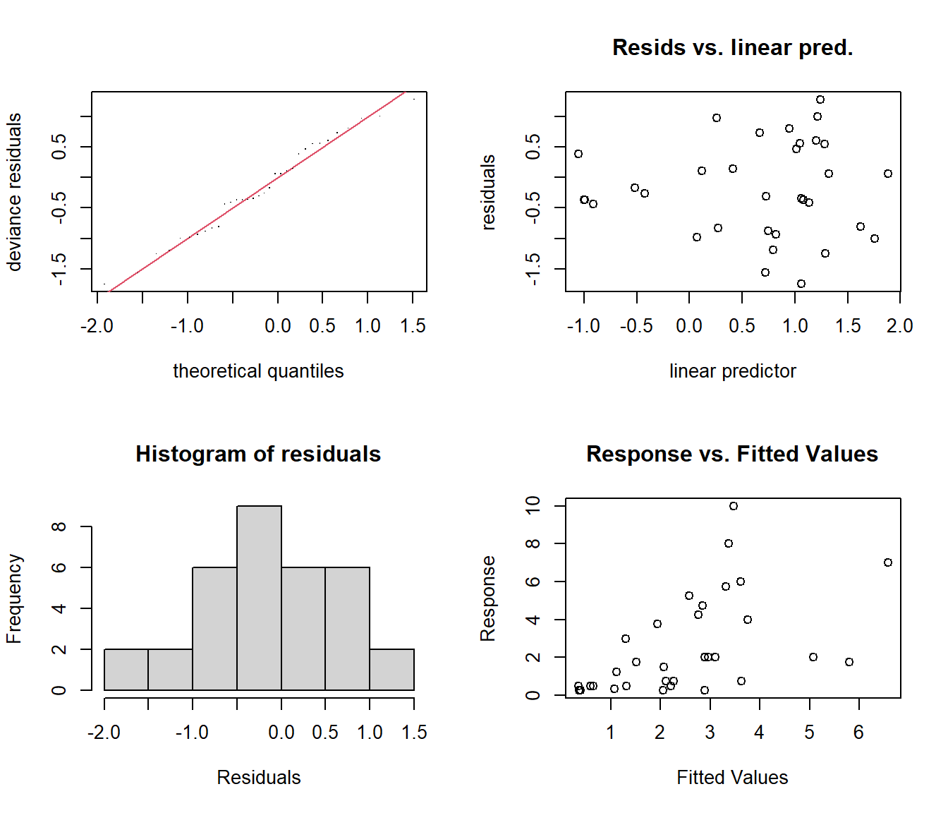
#| fig-height: 6
# Basis dimension check and residual diagnostics
gam.check(final_cpue_pos)
```
```{r}
#| label: cpue-pos-concurvity
#| include: true
# Concurvity — values approaching 1 indicate potential instability
concurvity(final_cpue_pos, full = FALSE)
```
### Model figure
```{r}
#| label: fig-cpue-hurdle
#| include: true
#| fig-width: 5.5
#| fig-height: 5
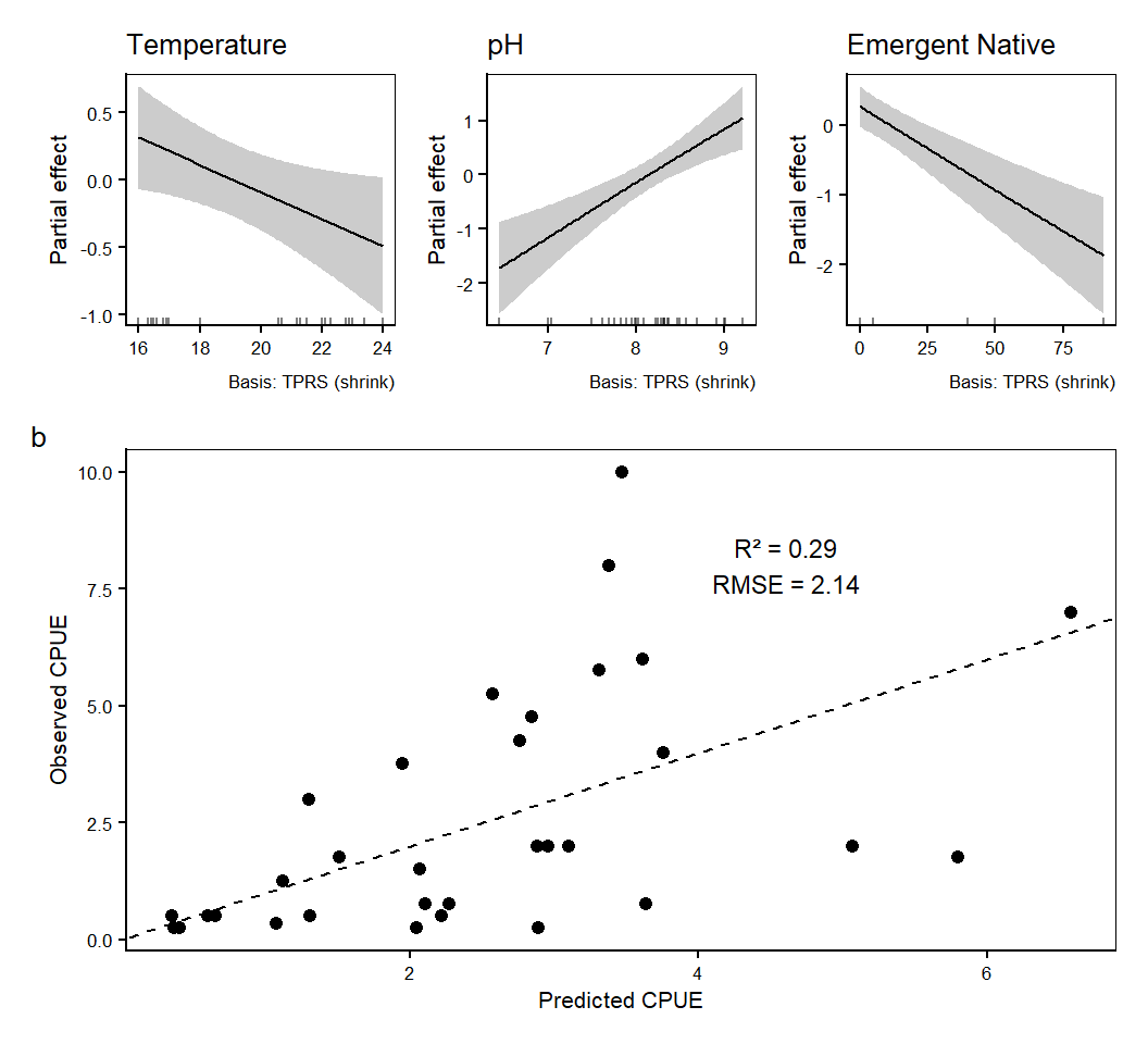
#| fig-cap: "Kōura CPUE GAMM results and model performance. (A) Estimated smooth terms for surface water temperature, pH, and emergent native macrophytes, shown with partial effects and 95% confidence intervals. See Fig. S2 for raw data underlying modelled relationships. (B) Predicted versus observed CPUE from the positive (Gamma) component of the hurdle model, with predictions excluding the random lake effect. The dashed 1:1 line indicates perfect agreement; annotated values report R² and RMSE to summarise model fit."
# make plot
sm_cpue <- smooth_estimates(final_cpue_pos)
cpue_smooth_names <- setdiff(unique(sm_cpue$.smooth), "s(LID)")
cpue_smooth_plots <- lapply(cpue_smooth_names, function(s) {
gratia::draw(final_cpue_pos, select = s, scales = "fixed", se = FALSE) +
labs(title = clean_smooth_title(s), x = NULL, y = "Partial effect") +
base_theme_bw
})

cpue_smooth_plots[[1]] <- cpue_smooth_plots[[1]] + labs(tag = "(A)")
p_cpue_pos_smooths <- patchwork::wrap_plots(cpue_smooth_plots, ncol = length(cpue_smooth_plots))

pred_pos <- predict(final_cpue_pos, type = "response")
obs_pos  <- final_cpue_pos$y
R2   <- cor(pred_pos, obs_pos, use = "complete.obs")^2
RMSE <- sqrt(mean((pred_pos - obs_pos)^2, na.rm = TRUE))

df_scat <- data.frame(Predicted = pred_pos, Observed = obs_pos)

p_cpue_pos_scatter <- ggplot(df_scat, aes(Predicted, Observed)) +
geom_point(size = 1.8, colour = "black") +
geom_abline(slope = 1, intercept = 0, linetype = "dashed", colour = "black", linewidth = 0.4) +
annotate(
"text",
x = max(df_scat$Predicted, na.rm = TRUE) * 0.7,
y = max(df_scat$Observed,  na.rm = TRUE) * 0.8,
label = paste0("R\u00B2 = ", round(R2, 2), "\nRMSE = ", round(RMSE, 2)),
size = 3
) +
labs(x = "Predicted CPUE", y = "Observed CPUE", tag = "(B)") +
base_theme_bw

CPUE_panel_positives <- (p_cpue_pos_smooths / p_cpue_pos_scatter) +
patchwork::plot_layout(heights = c(1, 2))

ggsave(filename = file.path(out_dir, "fig-cpue-hurdle.png"),plot = CPUE_panel_positives,width = 5.5, height = 5, dpi = 1200)

CPUE_panel_positives
```
## BPUE hurdle model
### Model fitting
```{r}
#| label: bpue-hurdle
#| include: false
BData <- prepare_block(Modeling_data, "Weighted_BPUE_Kōura", vars_common) %>%
dplyr::mutate(BPUE_pos = as.integer(Weighted_BPUE_Kōura > 0))

id <- "LID"

pred_fixed_BPUE_pres <- setdiff(names(BData),c("BPUE_pos", id, "Weighted_BPUE_Kōura", "Weighted_BPUE_Koura", "Weighted_BPUE"))

Bpos <- dplyr::filter(BData, BPUE_pos == 1L)

pred_fixed_BPUE_pos <- setdiff(names(Bpos), c("Weighted_BPUE_Kōura", id))

vif_BPUE_pos <- remove_high_vif_glmmTMB(Bpos,"Weighted_BPUE_Kōura",pred_fixed_BPUE_pos,threshold = vif_thresh,protect_vars = character(0))
kept_fixed_BPUE_pos <- vif_BPUE_pos$predictors

vars_step_BPUE_pos <- c(kept_fixed_BPUE_pos, if (INCLUDE_RE) id)

rhs_BPUE_pos <- paste(vapply(vars_step_BPUE_pos,function(v) build_smooth_gam(v, Bpos, custom_k, include_re_for_LID = INCLUDE_RE),
character(1)),
collapse = " + "
)

full_ml_BPUE_pos <- mgcv::gam(
as.formula(paste("Weighted_BPUE_Kōura ~", rhs_BPUE_pos)),
data   = Bpos,
family = Gamma(link = "log"),
method = "ML",
select = TRUE
)

remaining_BPUE_pos <- vars_step_BPUE_pos
protected_step_vars_bpos <- if (INCLUDE_RE) id else character(0)

repeat {
rhs_now <- paste(
vapply(
remaining_BPUE_pos,
function(v) build_smooth_gam(v, Bpos, custom_k, include_re_for_LID = INCLUDE_RE),
character(1)
),
collapse = " + "
)
m_now <- mgcv::gam(
as.formula(paste("Weighted_BPUE_Kōura ~", rhs_now)),
data   = Bpos,
family = Gamma(link = "log"),
method = "ML",
select = TRUE
)
sm <- summary(m_now)

ps <- c()
if (!is.null(sm$p.table) && nrow(sm$p.table) > 0) {
pcol <- intersect(colnames(sm$p.table), c("Pr(>|t|)", "Pr(>|z|)"))[1]
pvec <- sm$p.table[, pcol]
ps   <- c(ps, pvec[names(pvec) != "(Intercept)"])
}
if (!is.null(sm$s.table) && nrow(sm$s.table) > 0) {
pvec <- sm$s.table[, "p-value"]
names(pvec) <- rownames(sm$s.table)
ps   <- c(ps, pvec)
}
drop_candidates <- ps[ps > p_cutoff_ml]
if (!length(drop_candidates)) { red_ml_BPUE_pos <- m_now; break }

ordered <- names(sort(drop_candidates, decreasing = TRUE))
ordered_vars <- vapply(
ordered,
function(x) if (grepl("^s\\(", x)) sub("^s\\(([^,]+).*\\)$", "\\1", x) else x,
character(1)
)

ordered_vars <- setdiff(ordered_vars, protected_step_vars_bpos)
if (!length(ordered_vars)) { red_ml_BPUE_pos <- m_now; break }

remove_v <- ordered_vars[1]
remaining_BPUE_pos <- setdiff(remaining_BPUE_pos, remove_v)
if (!length(remaining_BPUE_pos)) { red_ml_BPUE_pos <- m_now; break }
}

final_bpue_pos <- mgcv::gam(
formula(red_ml_BPUE_pos),
data   = Bpos,
family = Gamma(link = "log"),
method = "REML",
select = TRUE
)
```
### Model diagnostics
```{r}
#| label: bpue-pos-diagnostics
#| include: true
#| fig-width: 7
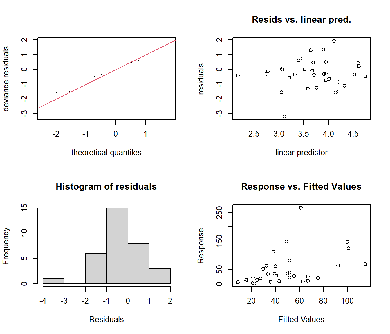
#| fig-height: 6
# Basis dimension check and residual diagnostics
gam.check(final_bpue_pos)
```
```{r}
#| label: bpue-pos-concurvity
#| include: true
# Concurvity — values approaching 1 indicate potential instability
concurvity(final_bpue_pos, full = FALSE)
```
### fig-bpue-hurdle
```{r}
#| label: fig-bpue-hurdle
#| include: true
#| fig-width: 4
#| fig-height: 5
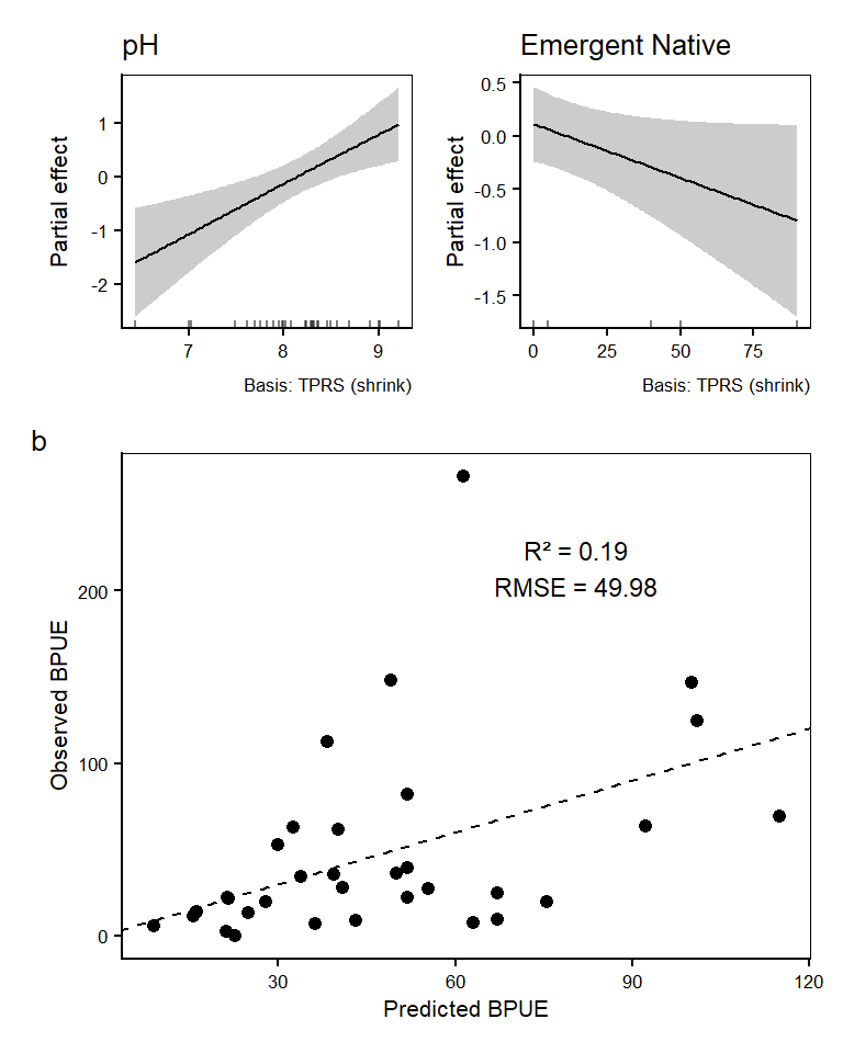
#| fig-cap: "Kōura BPUE GAMM results and model performance. (A) Estimated smooth terms for pH and emergent native macrophytes, shown with partial effects and 95% confidence intervals. See Fig. S2 for raw data underlying modelled relationships. (B) Predicted versus observed BPUE from the positive (Gamma) component of the hurdle model, with predictions excluding the random lake effect. The dashed 1:1 line indicates perfect agreement; annotated values report R² and RMSE to summarise model fit."
sm_bpue <- smooth_estimates(final_bpue_pos)
bpue_smooth_names <- setdiff(unique(sm_bpue$.smooth), "s(LID)")
bpue_smooth_plots <- lapply(bpue_smooth_names, function(s) {
gratia::draw(final_bpue_pos, select = s, scales = "fixed", se = FALSE) +
labs(title = clean_smooth_title(s), x = NULL, y = "Partial effect") +
base_theme_bw
})

bpue_smooth_plots[[1]] <- bpue_smooth_plots[[1]] + labs(tag = "(A)")
p_BPUE_pos_smooths <- patchwork::wrap_plots(bpue_smooth_plots, ncol = length(bpue_smooth_plots))

pred_pos_b <- predict(final_bpue_pos, type = "response")
obs_pos_b  <- final_bpue_pos$y
R2_b   <- cor(pred_pos_b, obs_pos_b, use = "complete.obs")^2
RMSE_b <- sqrt(mean((pred_pos_b - obs_pos_b)^2, na.rm = TRUE))

df_scat_b <- data.frame(Predicted = pred_pos_b, Observed = obs_pos_b)

p_BPUE_pos_scatter <- ggplot(df_scat_b, aes(Predicted, Observed)) +
geom_point(size = 1.8, colour = "black") +
geom_abline(slope = 1, intercept = 0, linetype = "dashed", colour = "black", linewidth = 0.4) +
annotate(
"text",
x = max(df_scat_b$Predicted, na.rm = TRUE) * 0.7,
y = max(df_scat_b$Observed,  na.rm = TRUE) * 0.8,
label = paste0("R\u00B2 = ", round(R2_b, 2), "\nRMSE = ", round(RMSE_b, 2)),
size = 3
) +
labs(x = "Predicted BPUE", y = "Observed BPUE", tag = "(B)") +
base_theme_bw

BPUE_panel_positives <- (p_BPUE_pos_smooths / p_BPUE_pos_scatter) +
patchwork::plot_layout(heights = c(1, 2))

ggsave(filename = file.path(out_dir, "fig-bpue-hurdle.png"),plot = BPUE_panel_positives,width = 4, height = 5, dpi = 1200)

BPUE_panel_positives
```
## Raw data plots all predictors
```{r}
#| label: fig-raw-data-all-predictors
#| fig-width: 5
#| fig-height: 10
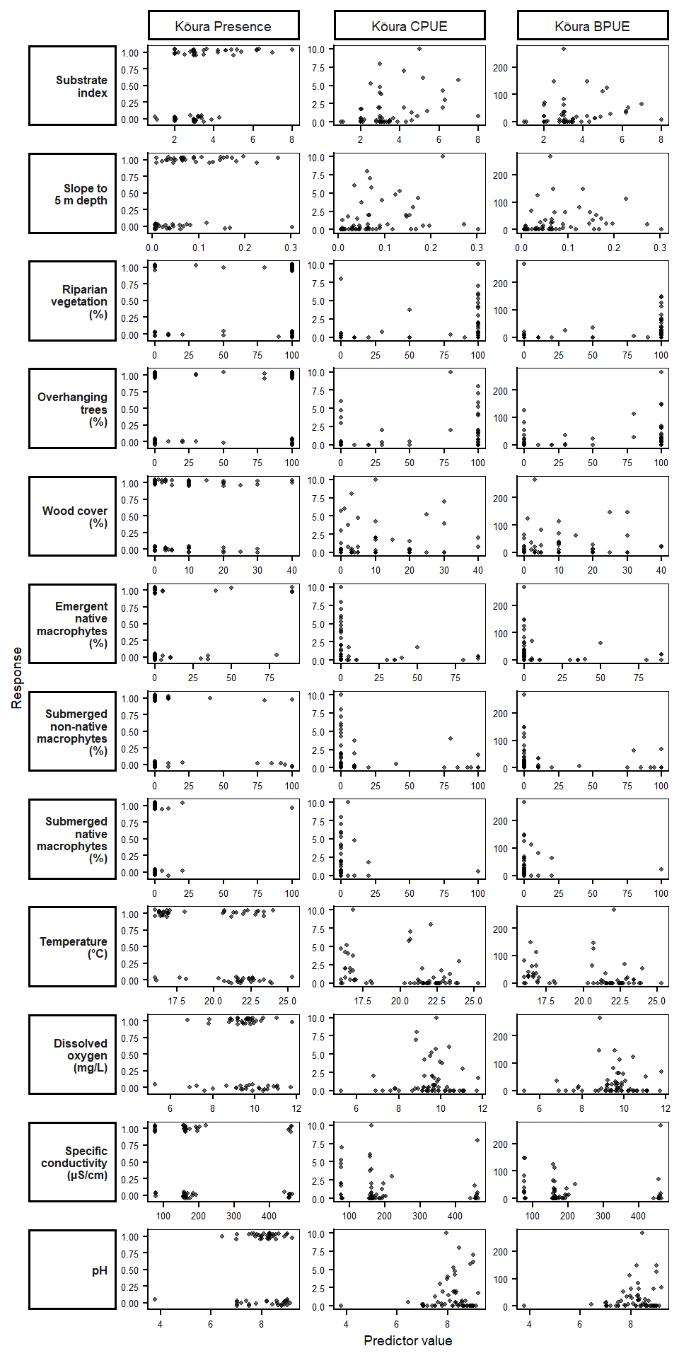
#| fig-cap: "Raw relationships between all environmental predictors examined and kōura occurrence, CPUE, and BPUE across all 60 surveyed littoral sites. Each panel shows observed values at individual sites (n = 60 for occurrence; n = 33 for CPUE and BPUE). Points are jittered slightly for occurrence data to reduce overplotting. Predictors highlighted in bold were retained in final GAM models."
# Variables examined across all models
all_pred_vars <- c(
  "Substrate_index", "Riparian_vegetation", "Temperature", "pH",
  "Specific_conductivity", "DO_mgl", "Slope_5m",
  "Overhanging_trees", "Wood_cover",
  "Emergent_Native", "Submerged_Non_Native", "Submerged_Native"
)

# Clean labels
pred_labels <- c(
  Substrate_index       = "Substrate\nindex",
  Slope_5m              = "Slope to\n5 m depth",
  Riparian_vegetation   = "Riparian\nvegetation\n(%)",
  Overhanging_trees     = "Overhanging\ntrees\n(%)",
  Wood_cover            = "Wood cover\n(%)",
  Emergent_Native       = "Emergent\nnative\nmacrophytes\n(%)",
  Submerged_Non_Native  = "Submerged\nnon-native\nmacrophytes\n(%)",
  Submerged_Native      = "Submerged\nnative\nmacrophytes\n(%)",
  Temperature           = "Temperature\n(°C)",
  DO_mgl                = "Dissolved\noxygen\n(mg/L)",
  Specific_conductivity = "Specific\nconductivity\n(µS/cm)",
  pH                    = "pH")

# Retained predictors (bold in strips)
retained_vars <- c("Substrate_index", "Riparian_vegetation", "Temperature",
                   "pH", "Specific_conductivity", "Emergent_Native")

# Build long-format data for all three responses
raw_long <- Monitoring_CPUE_data %>%
  dplyr::select(all_of(c(all_pred_vars,
                          "Presence_Kōura",
                          "Weighted_CPUE_Kōura",
                          "Weighted_BPUE_Kōura"))) %>%
  tidyr::pivot_longer(
    cols      = all_of(all_pred_vars),
    names_to  = "Predictor",
    values_to = "Predictor_value"
  ) %>%
  tidyr::pivot_longer(
    cols      = c("Presence_Kōura", "Weighted_CPUE_Kōura", "Weighted_BPUE_Kōura"),
    names_to  = "Response",
    values_to = "Response_value"
  ) %>%
  dplyr::mutate(
    Predictor_label = factor(pred_labels[Predictor], levels = pred_labels),
    Response        = dplyr::recode(Response,
      "Presence_Kōura"        = "Kōura Presence",
      "Weighted_CPUE_Kōura"   = "Kōura CPUE",
      "Weighted_BPUE_Kōura"   = "Kōura BPUE"
    ),
    Response = factor(Response, levels = c("Kōura Presence", "Kōura CPUE", "Kōura BPUE")),
    is_retained = Predictor %in% retained_vars
  )

# Strip label face: bold for retained predictors
strip_faces <- ifelse(levels(raw_long$Predictor_label) %in% pred_labels[retained_vars],"bold", "plain")

fig_raw_all <- ggplot(raw_long, aes(x = Predictor_value, y = Response_value)) +
  geom_jitter(
    data   = ~ dplyr::filter(.x, Response == "Kōura Presence"),
    height = 0.05, width = 0, size = 0.8, alpha = 0.6, colour = "black"  ) +
  geom_point(
    data   = ~ dplyr::filter(.x, Response != "Kōura Presence"),
    size   = 0.8, alpha = 0.6, colour = "black"  ) +
  ggh4x::facet_grid2(
    Predictor_label ~ Response,
    scales      = "free",
    independent = "all",
    switch      = "y"  ) +
  labs(x = "Predictor value", y = "Response") +
  base_theme_bw +
  theme(
    strip.text.y.left = element_text(size = 6, lineheight = 0.9, face = strip_faces, angle = 0, hjust = 1), strip.text.x      = element_text(size = 7),
    strip.placement   = "outside",
    axis.text         = element_text(size = 5),
    axis.title        = element_text(size = 7),
    panel.spacing     = unit(0.3, "lines")  )
fig_raw_all
ggsave(file.path(out_dir, "fig-raw-data-all-predictors.png"),
       fig_raw_all, width = 5, height = 10, dpi = 300)
```
## Full vs. reduced model comparison
```{r}
#| label: tbl-model-comparison
#| include: true
#| tbl-cap: "Comparison of full and stepwise-reduced (ML-fitted) models for kōura occupancy, CPUE, and BPUE, including AIC, likelihood ratio test (LRT) results, and the percentage deviance explained by the full, reduced, and final (REML-refitted) models."
compare_full_reduced <- function(full_model, reduced_model, final_model, model_name) {
  lrt <- anova(reduced_model, full_model, test = "LRT")

  tibble::tibble(
    model       = model_name,
    aic_full    = AIC(full_model),
    aic_reduced = AIC(reduced_model),
    lrt_chisq   = lrt[["Deviance"]][2],
    lrt_df      = lrt[["Df"]][2],
    lrt_p       = lrt[["Pr(>Chi)"]][2],
    dev_full    = summary(full_model)$dev.expl * 100,
    dev_reduced = summary(reduced_model)$dev.expl * 100,
    dev_final   = summary(final_model)$dev.expl * 100,
    r2_full     = summary(full_model)$r.sq,
    r2_reduced  = summary(reduced_model)$r.sq,
    r2_final    = summary(final_model)$r.sq
  )
}

model_comparison <- bind_rows(
  compare_full_reduced(full_ml_occ,      red_ml_occ,      final_occ,      "Occupancy"),
  compare_full_reduced(full_ml_cpue_pos, red_ml_cpue_pos, final_cpue_pos, "CPUE (pos)"),
  compare_full_reduced(full_ml_BPUE_pos, red_ml_BPUE_pos, final_bpue_pos, "BPUE (pos)")
)

write.csv(model_comparison, file = file.path(out_dir, "tbl-model-comparison.csv"), row.names = FALSE)

# Pull a value from model_comparison for inline reporting, e.g. mc_val("CPUE (pos)", "dev_final")
mc_val <- function(model_name, col) {
  model_comparison[[col]][model_comparison$model == model_name]
}

model_comparison |>
  mutate(
    across(c(aic_full, aic_reduced, lrt_chisq, lrt_df, dev_full, dev_reduced, dev_final, r2_full, r2_reduced, r2_final), ~ round(.x, 3)),
    lrt_p = format.pval(lrt_p, digits = 3, eps = 0.001)
  ) |>
  kable(
    col.names = c("Model", "AIC (full)", "AIC (reduced)", "LRT χ²", "LRT df", "LRT p-value",
                   "Deviance expl. full (%)", "Deviance expl. reduced (%)", "Deviance expl. final (%)",
                   "Adj. R² (full)", "Adj. R² (reduced)", "Adj. R² (final)"),
    align = c("l","r","r","r","r","r","r","r","r","r","r","r")
  )
```
## GAM model summary table
```{r}
#| label: tbl-gam-models
#| include: true
#| tbl-cap: "GAM model results for kōura occupancy, CPUE, and BPUE models. Significance codes: *** p < 0.001, ** p < 0.01, * p < 0.05, . p < 0.1"
gam_results_table <- function(model, model_name = deparse(substitute(model)), digits = 3) {
sm <- summary(model)

ptab <- as.data.frame(sm$p.table)
ptab <- rownames_to_column(ptab, "term")
ptab <- as_tibble(ptab)

p_col <- names(ptab)[grepl("^Pr\\(>\\|", names(ptab))]
if (length(p_col) != 1) stop("Could not uniquely identify p-value column in p.table.")

stat_col <- names(ptab)[grepl("value$", names(ptab))]
if (length(stat_col) != 1) stop("Could not uniquely identify statistic column in p.table.")

param_tbl <- ptab |>
rename(
estimate  = Estimate,
std_error = `Std. Error`,
statistic = all_of(stat_col),
p_value   = all_of(p_col)
) |>
mutate(component = "parametric", model = model_name) |>
select(model, component, term, estimate, std_error, statistic, p_value) |>
mutate(across(where(is.numeric), ~ round(.x, digits)))

stab <- as.data.frame(sm$s.table)
stab <- rownames_to_column(stab, "term")
stab <- as_tibble(stab)

refdf_col <- names(stab)[grepl("^Ref\\.df$", names(stab))]
edf_col   <- names(stab)[grepl("^edf$", names(stab))]
pval_col  <- names(stab)[grepl("^p\\-value$", names(stab))]
stat_col2 <- names(stab)[grepl("^(F|Chi\\.sq)$", names(stab))]

if (length(edf_col) != 1) stop("Could not uniquely identify edf column in s.table.")
if (length(refdf_col) != 1) stop("Could not uniquely identify Ref.df column in s.table.")
if (length(pval_col) != 1) stop("Could not uniquely identify p-value column in s.table.")
if (length(stat_col2) != 1) stop("Could not uniquely identify test statistic column in s.table.")

smooth_tbl <- stab |>
rename(
edf = all_of(edf_col),
ref_df = all_of(refdf_col),
statistic = all_of(stat_col2),
p_value = all_of(pval_col)) |>
mutate(component = "smooth", model = model_name) |>
select(model, component, term, edf, ref_df, statistic, p_value) |>
mutate(across(where(is.numeric), ~ round(.x, digits)))

combined_tbl <- bind_rows(
param_tbl |>
mutate(edf = NA_real_, ref_df = NA_real_) |>
select(model, component, term, estimate, std_error, edf, ref_df, statistic, p_value),
smooth_tbl |>
mutate(estimate = NA_real_, std_error = NA_real_) |>
select(model, component, term, estimate, std_error, edf, ref_df, statistic, p_value)
)

list(parametric = param_tbl, smooth = smooth_tbl, combined = combined_tbl)
}

occ_tabs  <- gam_results_table(final_occ,      "Occupancy", digits = 3)
cpue_tabs <- gam_results_table(final_cpue_pos, "CPUE (pos)", digits = 3)
bpue_tabs <- gam_results_table(final_bpue_pos, "BPUE (pos)", digits = 3)

add_sig <- function(df) {
df |>
mutate(
sig = case_when(
is.na(p_value) ~ "",
p_value < 0.001 ~ "***",
p_value < 0.01  ~ "**",
p_value < 0.05  ~ "*",
p_value < 0.1   ~ ".",
TRUE ~ ""
)
)
}

occ_table  <- add_sig(occ_tabs$combined)
cpue_table <- add_sig(cpue_tabs$combined)
bpue_table <- add_sig(bpue_tabs$combined)


all_models_table <- bind_rows(occ_table, cpue_table, bpue_table)
write.csv(all_models_table, file = file.path(out_dir, "tbl-gam-models.csv"), row.names = FALSE)

gam_models_table <- all_models_table |>
  mutate(
    term    = gsub("^s\\((.+)\\)$", "\\1", term),
    p_value = ifelse(!is.na(p_value), format.pval(p_value, digits = 3, eps = 0.001), NA)
  ) |>
  kable(col.names = c("Model", "Component", "Term", "Estimate", "SE", "EDF", "Ref.df", "Statistic", "p-value", ""),
    align = c("l","l","l","r","r","r","r","r","r","l"))

# Returns the comparison operator and the italic "p" label baked in
# (e.g. "*p* < 0.001" or "*p* = 0.023"). Set label = FALSE for values chained
# after a leading "*p*" (e.g. "*p* < 0.001, 0.011, 0.004, respectively").
get_pval <- function(model_name, term_name, component = "smooth", label = TRUE) {
  p_value <- all_models_table |>
    dplyr::filter(
      model     == model_name,
      grepl(term_name, term, fixed = TRUE),
      component == component
    ) |>
    dplyr::pull(p_value)

  out <- ifelse(p_value < 0.001, "< 0.001",
                paste0("= ", format.pval(p_value, digits = 3, eps = 0.001)))
  if (label) paste0("*p* ", out) else out
}

gam_models_table
```
# PCA (habitat complexity)
```{r}
#| label: pca
#| include: false
# Comment Frank about the modeling:
  # If you centered (on the mean) and standardized (scaled to unit variance) the predictors you could use the parameter estimates as an effect size to say something about the importance of the predictors (i.e. weak vs strong effects).


habitat_vars <- M_C_data %>%
dplyr::select(
Riparian_vegetation,
Substrate_index,
Wood_cover,
Overhanging_trees,
Emergent_Native,
Submerged_Native,
Submerged_Non_Native
) %>%
dplyr::filter(complete.cases(.))

habitat_pca <- prcomp(habitat_vars, center = TRUE, scale. = TRUE)

summary(habitat_pca)
biplot(habitat_pca)
habitat_pca$rotation
```
# Koura catfish interaction
```{r}
#| label: koura-catfish-interaction
#| include: false
# 1. Catfish distribution across habitat types
M_C_data %>%
  group_by(Habitat_Type) %>%
  summarise(n_sites = n(),
            catfish_present = sum(Presence_Catfish, na.rm = TRUE),
            koura_present = sum(Presence_Kōura, na.rm = TRUE),
            mean_CPUE_koura = mean(Weighted_CPUE_Kōura, na.rm = TRUE))
# 2. Kōura metrics: catfish-present vs absent sites
M_C_data %>%
  group_by(Presence_Catfish) %>%
  summarise(n = n(),
            koura_presence_rate = mean(Presence_Kōura, na.rm = TRUE),
            mean_CPUE_koura = mean(Weighted_CPUE_Kōura, na.rm = TRUE),
            mean_BPUE_koura = mean(Weighted_BPUE_Kōura, na.rm = TRUE))
# 3. Kōura metrics: catfish-invaded vs catfish-free lakes
M_C_data %>%
  mutate(catfish_lake = if_else(lake %in% c("Rotorua", "Rotoiti"),
                                "Catfish present", "Catfish absent")) %>%
  group_by(catfish_lake) %>%
  summarise(n_sites = n(),
            koura_presence_rate = mean(Presence_Kōura, na.rm = TRUE),
            mean_CPUE_koura = mean(Weighted_CPUE_Kōura, na.rm = TRUE),
            mean_BPUE_koura = mean(Weighted_BPUE_Kōura, na.rm = TRUE))
```
# Interactive widgets (saved as RDS for HTML thesis)
```{r}
#| label: widget-lake-overview-ch3
#| include: false
widget_lake_ov_rds <- file.path(der_data_dir, "widget_lake_overview.rds")
if (!file.exists(widget_lake_ov_rds)) {
  dt_w <- DT::datatable(
    lake_data, rownames = FALSE,
    options = list(pageLength = 12, dom = 'ft', scrollX = TRUE, autoWidth = TRUE)
  )
  saveRDS(dt_w, widget_lake_ov_rds)
}
```
```{r}
#| label: widget-site-map-ch3
#| include: false
widget_site_map_rds <- file.path(der_data_dir, "widget_site_map.rds")
if (!file.exists(widget_site_map_rds)) {
  study_lakes_w   <- c("Rotorua", "Rotoiti", "Rotoehu", "Rotomā", "Ōkāreka")
  catfish_lakes_w <- c("Rotorua", "Rotoiti")
  lakes_w <- sf::st_read("data/raw/12_lakes.gpkg", quiet = TRUE) |>
    sf::st_make_valid() |>
    sf::st_transform(4326)
  non_geom_w <- names(lakes_w)[!sapply(lakes_w, inherits, what = "sfc")]
  name_col_w <- if ("name" %in% non_geom_w && any(!is.na(lakes_w[["name"]]))) "name" else "name_ascii"
  lakes_w <- dplyr::rename(lakes_w, lake_name = dplyr::all_of(name_col_w))
  lakes_w <- dplyr::mutate(lakes_w,
    lake_name = sub("^Lake\\s+", "", lake_name),
    lake_name = trimws(sub("\\s*[/(\\&].*$", "", lake_name)),
    lake_name = dplyr::case_when(
      grepl("kareka", lake_name, ignore.case = TRUE) ~ "Ōkāreka",
      grepl("^Rotoma$", lake_name, ignore.case = TRUE) ~ "Rotomā",
      TRUE ~ lake_name
    )
  ) |>
    dplyr::filter(lake_name %in% study_lakes_w) |>
    dplyr::mutate(catfish = lake_name %in% catfish_lakes_w)
  sites_w <- readr::read_csv(file.path(der_data_dir, "Site_info.csv"), show_col_types = FALSE) |>
    dplyr::distinct(site_id, lake, lat, lon, DHT)
  dht_colors_w <- c("Rocky" = "#808080", "Sandy" = "#d4a843",
                     "Muddy" = "#8B6914", "Emergent Macrophyte" = "#228B22")
  sites_w <- dplyr::mutate(sites_w,
    color = dplyr::case_when(
      grepl("rocky",      DHT, ignore.case = TRUE) ~ "#808080",
      grepl("sandy",      DHT, ignore.case = TRUE) ~ "#d4a843",
      grepl("muddy",      DHT, ignore.case = TRUE) ~ "#8B6914",
      grepl("macrophyte", DHT, ignore.case = TRUE) ~ "#228B22",
      TRUE ~ "#555555"
    )
  )
  site_map_w <- leaflet::leaflet() |>
    leaflet::addProviderTiles("Esri.WorldGrayCanvas") |>
    leaflet::addPolygons(
      data = lakes_w, fillColor = ~ifelse(catfish, "#ffe0b2", "#e3f2fd"),
      fillOpacity = 0.5, color = "#2a2a2a", weight = 1.5,
      label = ~paste0(lake_name, ifelse(catfish, " (catfish present)", "")),
      popup = ~paste0("<b>", lake_name, "</b>", ifelse(catfish, "<br><i>Catfish present</i>", ""))
    ) |>
    leaflet::addCircleMarkers(
      data = sites_w, lat = ~lat, lng = ~lon, radius = 6,
      color = ~color, fillColor = ~color, fillOpacity = 0.9, weight = 1.5,
      popup = ~paste0("Site ", site_id, "<br>Lake: ", lake, "<br>Habitat: ", DHT)
    ) |>
    leaflet::addLegend(position = "bottomright", colors = unname(dht_colors_w),
                       labels = names(dht_colors_w), title = "Dominant habitat type", opacity = 0.9)
  saveRDS(site_map_w, widget_site_map_rds)
}
```
```{r}
#| label: widget-biotic-table-ch3
#| include: false
widget_biotic_rds <- file.path(der_data_dir, "widget_biotic_table.rds")
if (!file.exists(widget_biotic_rds)) {
  dt_w <- DT::datatable(biotic_vars, rownames = FALSE, filter = "top",
                        options = list(pageLength = 20, dom = 'frtip', scrollX = TRUE))
  saveRDS(dt_w, widget_biotic_rds)
}
```
# Session info
```{r}
#| label: session-info
#| include: true
#| code-fold: true
sessionInfo()
```